CCA-based celltype label transfer (scRNA → scATAC)#
Reproduces ArchR’s addGeneIntegrationMatrix workflow: canonical
correlation analysis (CCA) between the scATAC gene-score matrix and a
matched scRNA reference, followed by kNN-based label transfer. This is
how ArchR’s bookdown figures get their HSC / Ery / GMP / B / T cell
type labels — they come from the Granja et al. 2019 BMMC scRNA
reference, not from the ATAC clustering itself.
Pipeline
Load the 3-sample BMMC ATAC gene-score AnnData (
pbmc_gene_act.h5ad, output oft_integrate.ipynb— ~10 k cells × 20 k genes).Load the Granja 2019 BMMC scRNA reference (
granja2019_bmmc_scrna.h5ad— 35,582 cells × 20,287 genes, withobs['BioClassification']hematopoietic labels).Normalise both; pick their shared HVGs.
Run
cca_py.run_cca_anndata(atac, rna, ...)→ both objects get a sharedobsm['X_cca'].kNN in CCA space → transfer the majority-vote
BioClassificationlabel from RNA to each ATAC cell.Save annotated ATAC + transfer-confidence scores.
The annotated ATAC from (6) feeds straight into TF footprint
analysis (t_footprint.ipynb) or any other per-celltype ATAC
workflow.
Part 1 · Setup#
import pathlib
import numpy as np
import pandas as pd
import anndata as ad
import scanpy as sc
import matplotlib.pyplot as plt
from collections import Counter
from scipy import sparse
from sklearn.neighbors import NearestNeighbors

import epione as epi

epi.pl.plot_set()

WORK = pathlib.Path.cwd() / 'data'
OUT  = pathlib.Path.cwd() / 'label_transfer'
OUT.mkdir(exist_ok=True)
└─ 🔬 Starting plot initialization...
  ├─ Apply Scanpy/matplotlib settings
  ├─ Custom font setup
  ├─ Suppress warnings
  ├─
___________      .__
\_   _____/_____ |__| ____   ____   ____
 |    __)_\____ \|  |/  _ \ /    \_/ __ \
 |        \  |_> >  (  <_> )   |  \  ___/
/_______  /   __/|__|\____/|___|  /\___  >
        \/|__|                  \/     \/

  ├─ 🔖 Version: 0.0.1rc1   📚 Tutorials: https://epione.readthedocs.io/
└─ ✅ plot_set complete.
Part 2 · Load scRNA reference#
The Granja 2019 BMMC scRNA RDS was converted to h5ad once (see
scripts/convert_granja2019.R next to the tutorials) — this cell
just reads the result.
rna = ad.read_h5ad('/scratch/users/steorra/data/archr_heme/granja2019_bmmc_scrna.h5ad')
print(rna)
print('\nBioClassification distribution:')
print(rna.obs['BioClassification'].value_counts().head(15))
AnnData object with n_obs × n_vars = 35582 × 20287
    obs: 'Group', 'nUMI_pre', 'nUMI', 'nGene', 'initialClusters', 'UMAP1', 'UMAP2', 'Clusters', 'BioClassification', 'Barcode'
    var: 'gene_name', 'gene_id', 'exonLength'

BioClassification distribution:
BioClassification
12_CD14.Mono.2    4222
22_CD4.M          3539
20_CD4.N1         2470
21_CD4.N2         2364
05_CMP.LMPP       2260
25_NK             2143
07_GMP            2097
24_CD8.CM         2080
11_CD14.Mono.1    1800
17_B              1711
02_Early.Eryth    1653
19_CD8.N          1521
01_HSC            1425
08_GMP.Neut       1050
06_CLP.1           903
Name: count, dtype: int64
Part 3 · Load the 3-sample ATAC gene-score matrix#
t_integrate built this at pbmc_gene_act.h5ad — one row per
ATAC cell, columns are gene-score values (ArchR-style
distance-weighted tile signal per gene). Barcodes are in
<sample>#<barcode> format.
atac = ad.read_h5ad(WORK / 'pbmc_gene_act.h5ad')
print(atac)
print('\nATAC obs cols:', list(atac.obs.columns))
# Barcodes already <sample>#<barcode>.
AnnData object with n_obs × n_vars = 10889 × 20109
    obs: 'n_fragment', 'frac_dup', 'frac_mito', 'sample', 'leiden'
    var: 'gene_name'
    obsm: 'X_lsi', 'X_lsi_harmony', 'X_umap'
    obsp: 'connectivities', 'distances'

ATAC obs cols: ['n_fragment', 'frac_dup', 'frac_mito', 'sample', 'leiden']
Part 4 · Preprocess both sides#
Standard pipeline:
normalise total counts + log1p
scanpy HVG per dataset
intersect HVG gene names — this is the shared feature set CCA projects into
ArchR does the same preprocessing via
FindVariableFeatures/NormalizeData inside
addGeneIntegrationMatrix.
# log-normalise both + large HVG union (more features → better CCA
# anchor quality than tight intersection).
for ad_obj, name in [(rna, 'RNA'), (atac, 'ATAC')]:
    sc.pp.normalize_total(ad_obj, target_sum=1e4)
    sc.pp.log1p(ad_obj)
    sc.pp.highly_variable_genes(ad_obj, n_top_genes=5000, subset=False)

# Union HVG: genes variable in either modality (Seurat SelectIntegrationFeatures).
hvg_union = sorted(
    set(rna.var_names[rna.var['highly_variable']]) |
    set(atac.var_names[atac.var['highly_variable']])
)
# Restrict to genes present in both.
shared = sorted(set(rna.var_names) & set(atac.var_names))
hvg_shared = [g for g in hvg_union if g in shared][:4000]
print(f'shared genes    : {len(shared):,}')
print(f'union HVG ∩ shared: {len(hvg_shared):,}')
normalizing counts per cell
finished (0:00:00)
extracting highly variable genes
finished (0:00:00)
--> added
    'highly_variable', boolean vector (adata.var)
    'means', float vector (adata.var)
    'dispersions', float vector (adata.var)
    'dispersions_norm', float vector (adata.var)
normalizing counts per cell
finished (0:00:00)
extracting highly variable genes
finished (0:00:00)
--> added
    'highly_variable', boolean vector (adata.var)
    'means', float vector (adata.var)
    'dispersions', float vector (adata.var)
    'dispersions_norm', float vector (adata.var)
shared genes    : 17,677
union HVG ∩ shared: 4,000
Part 5 · Run CCA#
cca_py.run_cca_anndata standardises each dataset on the shared
HVG set, does a thin SVD on X^T @ Y, and writes the left / right
canonical factors back to each object’s obsm['X_cca']. 30
components is the ArchR default.
%%time
# ``epi.tl.integrate`` with method='cca' runs CCA on the shared HVG set
# and writes the L2-normalised canonical embedding to
# ``obsm[key_added]`` on both objects — ArchR ``addGeneIntegrationMatrix``
# (Seurat ``FindTransferAnchors(reduction='cca')``) analogue.
epi.tl.integrate(
    atac, rna,
    method='cca',
    features=hvg_shared,
    num_cc=30,
)
print(f'ATAC X_cca: {atac.obsm["X_cca"].shape}')
print(f'RNA  X_cca: {rna.obsm["X_cca"].shape}')
ATAC X_cca: (10889, 30)
RNA  X_cca: (35582, 30)
CPU times: user 5min 11s, sys: 4.01 s, total: 5min 15s
Wall time: 32.4 s
Part 6 · kNN label transfer#
For each ATAC cell, find its k=30 nearest RNA cells in CCA space
and assign the majority-vote BioClassification label. Record
the vote fraction as a transfer confidence score — values < 0.5
flag cells where the top celltype narrowly won; these are usually
ATAC cells sitting between two RNA clusters and worth treating with
caution downstream.
%%time
# ``epi.tl.transfer_labels`` does kNN in the shared CCA space and
# weighted-votes each query cell's label from its k nearest reference
# cells. Saves the kNN indices to obsm so the composition plot below
# can reuse them without recomputing.
epi.tl.transfer_labels(
    atac, rna, reference_label='BioClassification',
    k=30, strip_prefix=r'^\d+_',
    raw_key='celltype_cca', neighbors_key='cca_neighbors',
)
print(atac.obs['celltype'].value_counts().head(10))
print('transfer_score:', atac.obs['transfer_score'].describe().round(3).to_dict())
celltype
CD14.Mono.2 1439
CD4.M 1110
CMP.LMPP 973
CD4.N1 832
Early.Eryth 813
CD4.N2 691
HSC 662
GMP 646
B 576
NK 499
Name: count, dtype: int64
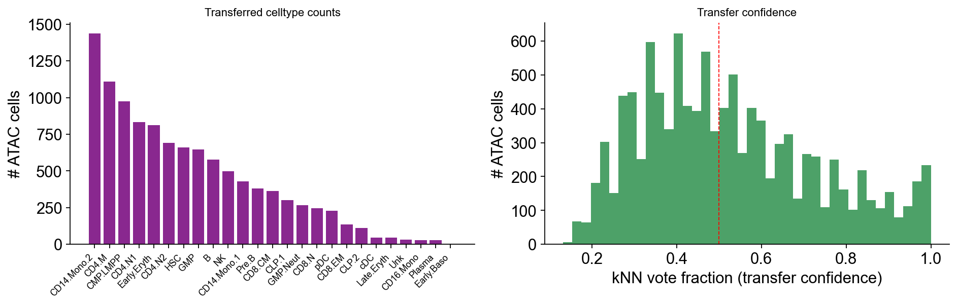
transfer_score: {'count': 10889.0, 'mean': 0.524, 'std': 0.207, 'min': 0.132, '25%': 0.364, '50%': 0.494, '75%': 0.664, 'max': 1.0}
CPU times: user 4.97 s, sys: 2.75 s, total: 7.72 s
Wall time: 5.44 s
# Collapse Granja fine BioClassification → ArchR bookdown coarse set
# (Clusters2). This mapping is dataset-specific (heme), so it lives
# in the tutorial, not the library.
COARSE_MAP = {
    'HSC':'HSC','CMP.LMPP':'CMP.LMPP','GMP':'GMP','GMP.Neut':'GMP',
    'CLP.1':'CLP','CLP.2':'CLP',
    'Early.Eryth':'Erythroid','Late.Eryth':'Erythroid','Pro.Eryth':'Erythroid',
    'CD14.Mono.1':'Mono','CD14.Mono.2':'Mono','CD16.Mono':'Mono',
    'pDC':'pDC','cDC':'cDC',
    'Pre.B':'PreB','B':'B','Plasma':'Plasma',
    'CD4.N1':'CD4.N','CD4.N2':'CD4.N','CD4.M':'CD4.M',
    'CD8.N':'CD8.N','CD8.CM':'CD8.CM','CD8.EM':'CD8.EM','NK':'NK',
}
atac.obs['celltype_coarse'] = (
    atac.obs['celltype'].astype(str).map(COARSE_MAP)
    .fillna(atac.obs['celltype'].astype(str))
)
print(atac.obs['celltype_coarse'].value_counts().head())
celltype_coarse
Mono        1898
CD4.N       1523
CD4.M       1110
CMP.LMPP     973
GMP          913
Name: count, dtype: int64
Part 7 · QC plots#
per-celltype cell counts
transfer-score distribution
optional: joint UMAP coloured by celltype
A well-behaved transfer shows a unimodal score distribution peaked near 1 (high confidence), with a long tail only for genuine inter- celltype boundary cells.
fig, (ax1, ax2) = plt.subplots(1, 2, figsize=(12, 4))
# Cell-count bar
counts = atac.obs['celltype'].value_counts()
ax1.bar(range(len(counts)), counts.values, color='#89288F')
ax1.set_xticks(range(len(counts)))
ax1.set_xticklabels(counts.index, rotation=45, ha='right', fontsize=8)
ax1.set_ylabel('# ATAC cells')
ax1.set_title('Transferred celltype counts', fontsize=10)
ax1.spines[['top','right']].set_visible(False)
# Score histogram
ax2.hist(atac.obs['transfer_score'], bins=40, color='#208A42', alpha=0.8)
ax2.set_xlabel('kNN vote fraction (transfer confidence)')
ax2.set_ylabel('# ATAC cells')
ax2.set_title('Transfer confidence', fontsize=10)
ax2.axvline(0.5, color='red', lw=0.8, ls='--')
ax2.spines[['top','right']].set_visible(False)
plt.tight_layout(); display(fig); plt.close(fig)
Part 7b · Joint UMAP of the CCA embedding#
ArchR’s bookdown shows the integration’s success by running UMAP on
the concatenated ATAC + RNA embedding and checking that cells of the
same type land together regardless of modality. We do the same here
— compute UMAP on the union of X_cca rows, colour by modality
(red=ATAC, blue=RNA) for the mixing view and by BioClassification
for the celltype view.
%%time
# ``epi.tl.joint_embedding`` concatenates ATAC + RNA on the shared CCA
# embedding, runs scanpy neighbours + UMAP, and returns the joint
# AnnData ready to plot.
joint = epi.tl.joint_embedding(
    atac, rna,
    use_rep='X_cca', labels=('ATAC', 'RNA'),
    label_columns=('celltype_coarse', 'BioClassification'),
    strip_prefix=r'^\d+_',
    n_neighbors=30, metric='cosine', random_state=0,
)
print(joint)
computing neighbors
finished: added to `.uns['neighbors']`
    `.obsp['distances']`, distances for each pair of neighbors
    `.obsp['connectivities']`, weighted adjacency matrix (0:00:40)
computing UMAP
finished: added
    'X_umap', UMAP coordinates (adata.obsm)
    'umap', UMAP parameters (adata.uns) (0:00:53)
AnnData object with n_obs × n_vars = 46471 × 17677
    obs: 'modality', 'celltype_joint'
    var: 'gene_name', 'gene_id', 'exonLength'
    uns: 'neighbors', 'umap'
    obsm: 'X_cca', 'X_umap'
    obsp: 'distances', 'connectivities'
CPU times: user 3min 51s, sys: 1.13 s, total: 3min 52s
Wall time: 1min 34s
# Two-panel UMAP: left = modality mixing (should intermix); right =
# celltype (same types cluster together across modalities).
fig, axes = plt.subplots(1, 2, figsize=(13, 5.5))
sc.pl.umap(joint, color='modality', size=6, ax=axes[0], show=False,
           title='Modality mixing (ATAC / RNA)', legend_loc='on data')
sc.pl.umap(joint, color='celltype_joint', size=6, ax=axes[1], show=False,
           title='Celltype', legend_loc='right margin', legend_fontsize=7)
plt.tight_layout(); display(fig); plt.close(fig)
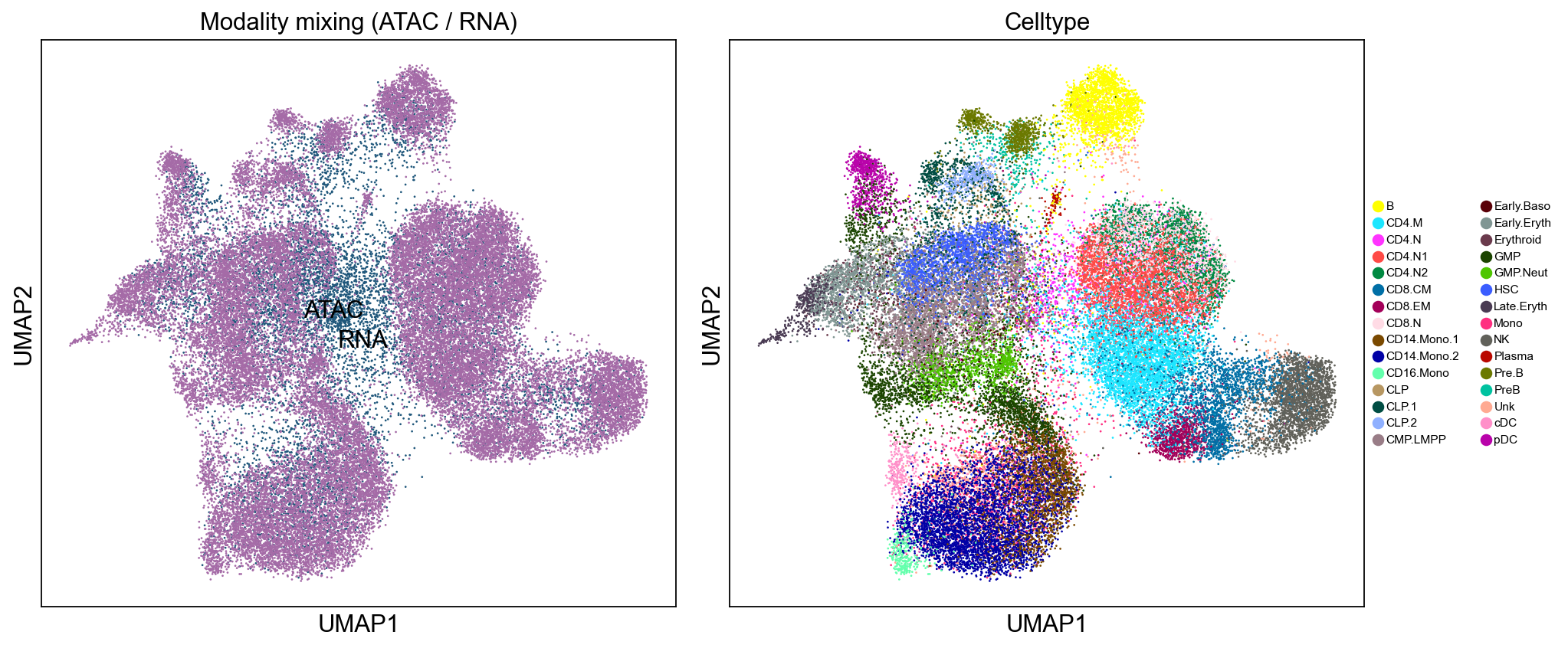
Reading the UMAP — in the left panel ATAC and RNA cells
should intermix freely (no ring-fenced ATAC-only islands, no
RNA-only islands); that’s the sign CCA has brought the two
modalities onto a common manifold. In the right panel, cells of
the same type should cluster together regardless of which modality
produced them. Any ATAC cells isolated from their RNA counterparts
are the low-confidence transfers flagged by the transfer_score < 0.5 threshold in Part 7.
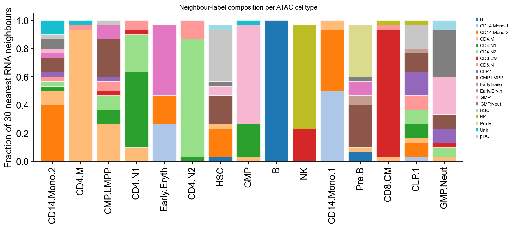
Part 7c · Label flow (RNA reference → ATAC)#
A Sankey-style bar visualises how each ATAC cell’s K nearest RNA cells distribute across BioClassification categories. A well-calibrated transfer gives a sharp mode per ATAC celltype (one tall bar per assignment).
# Reuse the kNN indices stashed on atac.obsm by transfer_labels.
idx = atac.obsm['cca_neighbors_idx']
rna_labels = rna.obs['BioClassification'].astype(str).str.replace(
    r'^\d+_', '', regex=True).to_numpy()
assigned = atac.obs['celltype'].astype(str).to_numpy()

# For each assigned celltype, average the neighbour-label composition.
comp = pd.DataFrame({
    lab: pd.Series(rna_labels[idx[i]]).value_counts(normalize=True)
    for i, lab in enumerate(assigned)
}).T.groupby(level=0).mean().fillna(0).T

top_assigned = atac.obs['celltype'].value_counts().head(15).index.tolist()
sub = comp[top_assigned].loc[(comp[top_assigned] > 0.05).any(axis=1)]

fig, ax = plt.subplots(figsize=(11, 5))
sub.T.plot.bar(stacked=True, ax=ax, colormap='tab20', width=0.85,
               edgecolor='white', lw=0.3)
ax.set_ylabel('Fraction of 30 nearest RNA neighbours')
ax.set_title('Neighbour-label composition per ATAC celltype', fontsize=10)
ax.legend(frameon=False, fontsize=7, bbox_to_anchor=(1.02, 1), loc='upper left')
ax.spines[['top','right']].set_visible(False)
plt.tight_layout(); display(fig); plt.close(fig)
Part 8 · Save annotated ATAC#
Write a compact AnnData carrying just obs/obsm/uns of the
annotated gene-score matrix (dropping X, since the raw gene
scores already live in pbmc_gene_act.h5ad). Downstream
footprint / peak-matrix workflows re-read fragments from
uns['files']['fragments'].
out_h5 = OUT / 'atac_bmmc_cca_annotated.h5ad'
keep = ad.AnnData(
    X=sparse.csr_matrix((atac.n_obs, 0), dtype=np.float32),
    obs=atac.obs[['sample','celltype','celltype_cca','celltype_coarse','transfer_score']].copy(),
    obsm={'X_cca': atac.obsm['X_cca']},
    uns={'files': {'fragments': 'data/pbmc_combined.fragments.tsv.gz'}},
)
keep.obs_names = atac.obs_names
keep.write_h5ad(out_h5)
print(f'saved {out_h5}  ({out_h5.stat().st_size/1e6:.1f} MB)')
print()
print('Sanity: celltype cross-tab with existing heuristic label (t_integrate):')
try:
    old = ad.read_h5ad(WORK / 'pbmc_peak_mat_anno.h5ad').obs.loc[atac.obs_names, 'celltype']
    print(pd.crosstab(old, atac.obs['celltype']))
except Exception as e:
    print('  (skipped —', e, ')')
saved /scratch/users/steorra/analysis/omicverse_dev/epione/epione_guide/tutorials/single/label_transfer/atac_bmmc_cca_annotated.h5ad  (2.3 MB)

Sanity: celltype cross-tab with existing heuristic label (t_integrate):
celltype     B  CD14.Mono.1  CD14.Mono.2  CD16.Mono  CD4.M  CD4.N1  CD4.N2  \
celltype
B cells    335            3            1          0     15      10       3
CLP         12           20           27          0     41      42      17
CMP_LMPP    22           35           88          6     50      45      16
Early Ery   11           15           15          0     43      31      18
Endo        12            4            4          0     22      32      18
HSC         24           20           32          2     80      86      36
Late Ery     9            6            7          0     21      24      11
Mono        64          311         1242         21     97      86      36
NK           2            2            3          0      1       5       3
NKT         25            4            4          0     25      19      14
T cells     14            2            6          0    640     408     495
pDC         12            1            4          0     19      22      10
pre-B       34            6            6          1     56      22      14

celltype   CD8.CM  CD8.EM  CD8.N  ...  GMP  GMP.Neut  HSC  Late.Eryth   NK  \
celltype                          ...
B cells         2       1      0  ...   18         2    1           1    2
CLP             7       1      6  ...   46        57   84           0   18
CMP_LMPP        9       3      6  ...  118        41   42           3   17
Early Ery       8       4     11  ...   29        24   85           5   13
Endo            1       0      3  ...    6         2   16           1    0
HSC            18       7     19  ...   76        22  269           1   34
Late Ery        2       0      4  ...   14        15   58          22    2
Mono           26      11     13  ...  193        65   56           5   33
NK             10       4      2  ...    4         0    2           0  214
NKT             3       1      5  ...   11         9   14           0    2
T cells        90      78    165  ...   52        22   20           8   45
pDC             3       1      2  ...   61         0   10           0    2
pre-B         184      24     10  ...   18         8    5           0  117

celltype   Plasma  Pre.B  Unk  cDC  pDC
celltype
B cells         4     29    1    2    3
CLP             3      7    1    0   10
CMP_LMPP        3     10    6   14   29
Early Ery       0      9    0    1    5
Endo            0      1    1    0    2
HSC             5     21    2    5   20
Late Ery        0      7    0    3    3
Mono            4      2   16   20   39
NK              0      1    1    0    0
NKT             1     88    0    0    3
T cells         5      5    3    0    2
pDC             0     12    0    2  111
pre-B           3    190    1    0    3

[13 rows x 25 columns]
Notes#
addGeneIntegrationMatrixin ArchR uses Seurat’sFindTransferAnchors(reduction='cca')→TransferData. We implement the same idea (CCA + kNN vote) withcca_py+sklearn.NearestNeighbors. The CCA embedding is deterministic givenseed=; reruns return identical labels.For even stronger transfer, weight the kNN votes by
1 / (1 + dist)instead of uniform majority.If you don’t have the Granja reference, any BMMC scRNA AnnData with a
BioClassification-like column will work — just pass it asrnain Part 2.