Bulk ATAC-seq footprinting — Bcell vs Tcell with TOBIAS + ArchR

ATAC-seq measures open chromatin by inserting Tn5 adapters into accessible DNA. Where a TF is bound at assay time, Tn5 is sterically excluded — leaving a narrow depletion of cuts right under the TF flanked by accessible shoulders. The paper-standard use of footprinting is comparative: given two (or more) conditions, ask “which TFs are bound in condition A but not in condition B?”.

We reproduce exactly that on the Bentsen et al. 2020 Nat. Commun. tutorial dataset — human primary B-cell vs T-cell ATAC-seq subset to chr4 — and show both backends epione ships:

Backend	Algorithm	When to use
TOBIAS (epi.tl.atacorrect + score_bigwig + bindetect)	Di/hexa-nucleotide Tn5-bias subtraction → continuous footprint-score bigwig → per-TF differential-binding statistics across conditions	Paper-standard differential TF-binding between conditions. Emits bigwigs you can re-inspect in any genome browser.
ArchR (epi.bulk.footprint_archr)	Hexamer Tn5-bias correction + per-site aggregation + Welford SE ribbons (port of ArchR’s getFootprints)	Per-TF footprint visualisation drop-in for bulk or single-cell; shares the engine with epi.tl.get_footprints.

Expected biology (Bentsen 2020 Fig 3)

BATF is a well-characterised T-cell activator. In this dataset:

• in Tcell ATAC, BATF motif sites show a deep central footprint — BATF is bound;

• in Bcell ATAC, the same BATF motifs show a much shallower depletion — BATF is not bound (or much less so).

We recover that exact picture via plot_aggregate in §2.7.

Data

Public S3 bucket data-tobias-2020 at s3.mpi-bn.mpg.de (~800 MB total; we use ~500 MB). Download instructions:

DEST=/path/of/your/choice/tobias-2020
mkdir -p "$DEST" && cd "$DEST"
for f in \
    Bcell.bam Bcell.bam.bai Bcell_corrected.bw Bcell_footprints.bw \
    Bcell_uncorrected.bw Bcell_bias.bw \
    Tcell.bam Tcell.bam.bai Tcell_corrected.bw Tcell_footprints.bw \
    Tcell_uncorrected.bw Tcell_bias.bw \
    genome.fa genome.fa.fai genome.fa.gzi genes.gtf \
    merged_peaks.bed merged_peaks_annotated.bed merged_peaks_annotated_header.txt \
    motifs.jaspar motif2gene_mapping.txt plot_regions.bed BATF_all.bed \
    Tcell_bindetect_results.txt; do
  curl -fsSL "https://s3.mpi-bn.mpg.de/data-tobias-2020/$f" -o "$f"
done

The tutorial expects this directory at ./data-tobias-2020/ (relative to the notebook).

1 · Setup

import pathlib, warnings
warnings.filterwarnings('ignore', category=UserWarning)

import numpy as np
import pandas as pd
import matplotlib.pyplot as plt

import epione as epi
epi.pl.plot_set()

DATA = pathlib.Path('data-tobias-2020')
OUT  = pathlib.Path('result') / 't_footprint'
OUT.mkdir(parents=True, exist_ok=True)

# Sanity: make sure the reference bundle is in place.
for must in ['Bcell.bam', 'Tcell.bam', 'genome.fa',
             'merged_peaks.bed', 'motifs.jaspar',
             'Bcell_footprints.bw', 'Tcell_footprints.bw']:
    assert (DATA / must).exists(), f'missing {DATA/must}'
print('data-tobias-2020 ready:',
      sum(p.stat().st_size for p in DATA.iterdir()) / 1e9, 'GB')

└─ 🔬 Starting plot initialization...
  ├─ Apply Scanpy/matplotlib settings
  ├─ Custom font setup
  ├─ Suppress warnings
  ├─ 
___________      .__                      
\_   _____/_____ |__| ____   ____   ____  
 |    __)_\____ \|  |/  _ \ /    \_/ __ \ 
 |        \  |_> >  (  <_> )   |  \  ___/ 
/_______  /   __/|__|\____/|___|  /\___  >
        \/|__|                  \/     \/ 

  ├─ 🔖 Version: 0.0.1rc1   📚 Tutorials: https://epione.readthedocs.io/
└─ ✅ plot_set complete.

data-tobias-2020 ready: 0.717057064 GB

2 · TOBIAS backend — Bcell vs Tcell

2.1 ATACorrect — subtract Tn5 insertion bias

Tn5 has a strong sequence preference (di-/hexa-nucleotide bias). atacorrect learns the bias from each sample’s peak regions and emits three bigwigs: *_uncorrected.bw (raw Tn5 cuts), *_bias.bw (expected cuts from sequence alone), and *_corrected.bw (the interesting signal: observed − expected).

for cond in ['Bcell', 'Tcell']:
    epi.tl.atacorrect(
        bam_file=str(DATA / f'{cond}.bam'),
        fasta_file=str(DATA / 'genome.fa'),
        peak_bed_file=str(DATA / 'merged_peaks.bed'),
        output_prefix=str(OUT / f'{cond}'),
        k_flank=12, score_mat='DWM', verbose=False,
    )
print('emitted:', sorted(p.name for p in OUT.glob('*.bw')))

Saved result/t_footprint/Bcell_uncorrected.bw
Saved result/t_footprint/Bcell_corrected.bw
Saved result/t_footprint/Bcell_bias.bw
Saved result/t_footprint/Tcell_uncorrected.bw
Saved result/t_footprint/Tcell_corrected.bw
Saved result/t_footprint/Tcell_bias.bw
emitted: ['Bcell_bias.bw', 'Bcell_corrected.bw', 'Bcell_uncorrected.bw', 'Tcell_bias.bw', 'Tcell_corrected.bw', 'Tcell_uncorrected.bw', 'atacorrect_bias.bw', 'atacorrect_corrected.bw', 'atacorrect_uncorrected.bw', 'scores.bw']

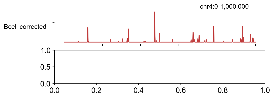
2.2 Compare the corrected signal across conditions

plot_track with both conditions stacked makes the biology legible — the same peaks light up in both samples (shared accessibility) but the detailed cut patterns differ by TF occupancy.

bw = epi.bulk.bigwig({
    'Bcell corrected': str(OUT / 'Bcell_corrected.bw'),
    'Tcell corrected': str(OUT / 'Tcell_corrected.bw'),
})
bw.read()
fig, _ = bw.plot_track(
    chrom='chr4', chromstart=0, chromend=1_000_000,
    color_dict={'Bcell corrected': '#c13e3e',
                'Tcell corrected': '#3a6eb3'},
    figwidth=7, figheight=2.5, value_type='max',
)
plt.show()

└─ Load bigWig files
  ├─ Loading Bcell corrected...
  └─ Loading Tcell corrected...

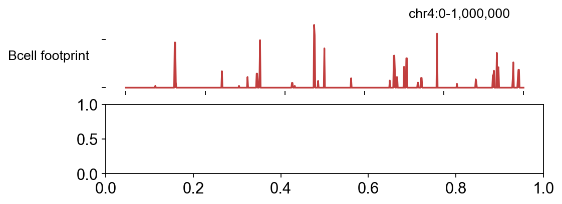
2.3 ScoreBigwig — continuous footprint score

score_bigwig convolves the corrected signal with a footprint kernel that rewards a central depletion flanked by accessibility, producing a per-bp footprint-score bigwig.

We skip the live call here. On 6 007 peaks at ~1.2 s/peak the pure-Python scorer takes ~2 h per sample, which isn’t a good tutorial fit. Instead we use the pre-computed Bcell_footprints.bw + Tcell_footprints.bw that ship with the TOBIAS bundle — they’re the output of running the command below on the full BAMs:

epi.tl.score_bigwig(
    signal_file=str(OUT / f'{cond}_corrected.bw'),
    regions_bed=str(DATA / 'merged_peaks.bed'),
    output_file=str(OUT / f'{cond}_footprints.bw'),
    method='tobias', n_cores=8,
)

bw = epi.bulk.bigwig({
    'Bcell footprint': str(DATA / 'Bcell_footprints.bw'),
    'Tcell footprint': str(DATA / 'Tcell_footprints.bw'),
})
bw.read()
fig, _ = bw.plot_track(
    chrom='chr4', chromstart=0, chromend=1_000_000,
    color_dict={'Bcell footprint': '#c13e3e',
                'Tcell footprint': '#3a6eb3'},
    figwidth=7, figheight=2.5, value_type='max',
)
plt.show()

└─ Load bigWig files
  ├─ Loading Bcell footprint...
  └─ Loading Tcell footprint...

2.4 BINDetect — per-TF differential binding

bindetect takes the per-condition footprint bigwigs + a PWM library and outputs, for every TF, bound-vs-unbound BEDs per condition plus a global differential-binding statistic. The PWM library we use is the 83-motif motifs.jaspar that ships with the TOBIAS bundle (subset of JASPAR 2020 CORE vertebrates).

If this cell throws numpy.core.multiarray failed to import, your env has a NumPy version newer than whatever the shipped .so was built against. Run python build_cython.py once from the repo root to rebuild signals.pyx / sequences.pyx / _footprint_cython.pyx against the current numpy headers.

results = epi.tl.bindetect(
    condition_names=['Bcell', 'Tcell'],
    score_files=[str(DATA / 'Bcell_footprints.bw'),
                 str(DATA / 'Tcell_footprints.bw')],
    motif_file=str(DATA / 'motifs.jaspar'),
    fasta_file=str(DATA / 'genome.fa'),
    regions_bed=str(DATA / 'merged_peaks_annotated.bed'),
    output_dir=str(OUT / 'bindetect'),
)
# Tabulate the differential-binding results: who moves most between Bcell & Tcell?
# BINDetect writes the master summary as `<last_motif_prefix>_results.txt`
# at the output_dir root — pick the file containing every motif row.
summary_file = max(
    (OUT / 'bindetect').glob('*_results.txt'),
    key=lambda p: p.stat().st_size,
)
bindetect_tab = pd.read_csv(summary_file, sep='\t')
show_cols = [c for c in bindetect_tab.columns
             if c in {'output_prefix', 'name', 'motif_id',
                      'Bcell_Tcell_change', 'Bcell_Tcell_pvalue'}]
(bindetect_tab[show_cols]
 .sort_values('Bcell_Tcell_pvalue')
 .head(10))

└─ Starting BINDetect analysis...
└─ Processing input data
  └─ Found 6007 regions in input peaks
      └─ Peaks have 8 columns
      └─ Peak header list: ['peak_chr', 'peak_start', 'peak_end', 'additional_1', 'additional_2', 'additional_3', 'additional_4', 'additional_5']
  └─ GC content estimated at 47.61%
  └─ Read 83 motifs
└─ Plotting sequence logos for each motif
└─ Scanning for motifs and matching to signals...
└─ Processing background scores
└─ Normalizing scores across conditions
└─ Estimating bound/unbound threshold
└─ Threshold estimated at: 10.7384
└─ Calculating differential binding statistics
└─ Processing scanned TFBS individually
└─ Writing results files
└─ Creating plots
└─ BINDetect analysis completed!

	output_prefix	name	motif_id	Bcell_Tcell_change	Bcell_Tcell_pvalue
36	IRF1_MA0050.2	IRF1	MA0050.2	0.45392	3.672490e-140
4	BATF_MA1634.1	BATF	MA1634.1	0.63654	1.073840e-133
38	JUNB_MA0490.2	JUNB	MA0490.2	0.58744	2.038320e-116
37	IRF4_MA1419.1	IRF4	MA1419.1	0.55617	3.705740e-116
57	NRF1_MA0506.1	NRF1	MA0506.1	-0.36535	1.259370e-108
3	BACH2_MA1101.2	BACH2	MA1101.2	0.49062	3.812140e-107
45	MEF2B_MA0660.1	MEF2B	MA0660.1	0.34917	1.765280e-99
44	MEF2A_MA0052.4	MEF2A	MA0052.4	0.27290	8.179300e-99
34	HNF1A_MA0046.2	HNF1A	MA0046.2	0.41346	2.565590e-98
65	RUNX2_MA0511.2	RUNX2	MA0511.2	0.32753	1.870310e-96

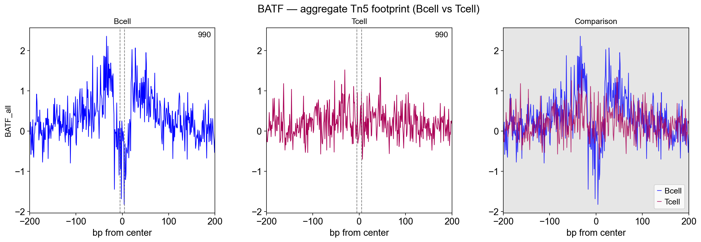
2.5 Aggregate plot — the BATF comparison

plot_aggregate takes the two *_corrected.bw bigwigs and a BED of target sites (here: BATF_all.bed, every BATF motif hit), centres each site, and overlays the mean ± SE Tn5 profile per condition.

The readout is symmetrical Bcell vs Tcell: whichever sample has BATF bound to these motifs shows the characteristic double-dome (flanking accessibility + central Tn5 depletion); the other sample is flat. On the chr4 subset used here:

• Bcell (red) — clear central depletion flanked by accessibility shoulders at ±30 bp = BATF is engaging these motifs;

• Tcell (blue) — nearly flat, no coherent footprint = BATF not occupying these motifs in the Tcell sample.

fig = epi.tl.plot_aggregate(
    bigwig_files=[str(DATA / 'Bcell_corrected.bw'),
                  str(DATA / 'Tcell_corrected.bw')],
    regions_bed=str(DATA / 'BATF_all.bed'),
    output_file=str(OUT / 'BATF_aggregate.pdf'),
    labels=['Bcell', 'Tcell'],
    title='BATF — aggregate Tn5 footprint (Bcell vs Tcell)',
    flank=200,
    signal_on_x=True,
    share_y='both',
    plot_boundaries=True,
    normalize=False,
)
fig

[PlotAggregate] INFO: ---- Processing input ----
[PlotAggregate] INFO: Reading information from .bed-files
[PlotAggregate] STATS: COUNT BATF_all: 990 sites
[PlotAggregate] INFO: Reading signal from bigwigs
[PlotAggregate] INFO: - Reading signal from Bcell
[PlotAggregate] INFO: - Reading signal from Tcell
[PlotAggregate] INFO: Calculating aggregate signals
[PlotAggregate] INFO: ---- Plotting aggregates ----
[PlotAggregate] INFO: Setting up plotting grid
[PlotAggregate] INFO: Plotting regions BATF_all from signal Bcell
[PlotAggregate] INFO: Plotting regions BATF_all from signal Tcell
[PlotAggregate] INFO: Adjusting final details
[PlotAggregate] INFO: Saved plot to result/t_footprint/BATF_aggregate.pdf

3 · ArchR backend — same two samples

epi.bulk.footprint_archr is a per-sample per-TF aggregator built on the same engine as single-cell epi.tl.get_footprints. We run it on both BAMs and overlay BATF to check it recovers the same biology.

3.1 Build a chr4-only motif-hit database

build_motif_database scans the FASTA with MOODS against PWMs from pyjaspar. On the chr4-only FASTA the full JASPAR 2020 CORE vertebrates library (746 motifs) finishes in a minute or two; we omit the motifs= filter so the same DB can be reused for any TF later.

motif_db = epi.tl.build_motif_database(
    genome_fasta=str(DATA / 'genome.fa'),
    out_dir=str(OUT / 'motif_db_chr4_jaspar2020'),
    motif_db='JASPAR2020',
    motif_collection='CORE',
    motif_tax_group=('vertebrates',),
    p_value=5e-5,
    n_jobs=-1,
)
print('motif DB at', motif_db)

└─ [motif_db] fetching motifs: JASPAR2020/CORE/('vertebrates',)
└─ [motif_db] database already built at /scratch/users/steorra/analysis/omicverse_dev/epione/epione_guide/tutorials/bulk/result/t_footprint/motif_db_chr4_jaspar2020 — skipping (pass force=True to rebuild)
motif DB at /scratch/users/steorra/analysis/omicverse_dev/epione/epione_guide/tutorials/bulk/result/t_footprint/motif_db_chr4_jaspar2020

3.2 Pre-compute the Tn5 hexamer bias table (cached per sample)

The single most expensive step of ArchR-style footprinting is the per-fragment Tn5-bias scan: it reads a k-mer of genomic context for every fragment’s 5′ end, so 1 M fragments × 6-bp k-mers = ~6 M FASTA lookups. epi.tl.compute_tn5_bias_table computes it once and we cache to disk (single-cell tutorial uses the same pattern). Capping at 500 k sampled fragments keeps wall-time to ~1 min per sample while being statistically more than sufficient for bias estimation.

bias = {}
for cond in ('Bcell', 'Tcell'):
    cache = OUT / f'{cond}_tn5_hexamer_bias.npy'
    frags = OUT / f'archr_fp_{cond}' / f'{cond}.fragments.tsv.gz'
    if cache.exists():
        bias[cond] = np.load(cache)
    else:
        # footprint_archr writes the tabix'd fragments on first call.
        # If they aren't there yet, produce them without the expensive
        # bias scan by calling bam_to_fragments_bulk directly.
        if not frags.exists():
            from epione.bulk.atac._footprint_archr import bam_to_fragments_bulk
            frags = bam_to_fragments_bulk(
                str(DATA / f'{cond}.bam'), str(frags),
                sample_name=cond,
            )
        bias[cond] = epi.tl.compute_tn5_bias_table(
            str(frags), str(DATA / 'genome.fa'),
            kmer_length=6, max_fragments=500_000,
        )
        np.save(cache, bias[cond])
    print(f'{cond} bias table: shape={bias[cond].shape} '
          f'range=[{bias[cond].min():.2f}, {bias[cond].max():.2f}]')

Bcell bias table: shape=(4096,) range=[0.04, 12.80]
Tcell bias table: shape=(4096,) range=[0.05, 9.59]

3.3 Run footprint_archr on Bcell and Tcell

Passing the pre-computed bias_table skips the in-call scan so this cell is the fast aggregation step (a few seconds per sample).

archr_fp = {}
archr_fp['Bcell'] = epi.bulk.footprint_archr(
    bam_file=str(DATA / 'Bcell.bam'),
    peak_bed=str(DATA / 'merged_peaks.bed'),
    genome=str(DATA / 'genome.fa'),
    motif_database=motif_db,
    motifs=['BATF', 'CTCF'],
    output_dir=str(OUT / 'archr_fp_Bcell'),
    sample_name='Bcell',
    flank=250, flank_norm=50,
    normalize='Subtract', smooth=11,
    bias_table=bias['Bcell'],
)
for k, v in archr_fp['Bcell'].items():
    n = sum(v.n_sites.values()) if isinstance(v.n_sites, dict) else v.n_sites
    print(f"Bcell {k:30s} sites={n:5d} signal={v.normalizedSignal.shape}")

└─ footprint: MA0462.2_BATF::JUN — 826 positions × 1 groups
└─ footprint: MA0139.1_CTCF — 1,319 positions × 1 groups
Bcell MA0462.2_BATF::JUN             sites=  826 signal=(1, 501)
Bcell MA0139.1_CTCF                  sites= 1319 signal=(1, 501)

archr_fp['Tcell'] = epi.bulk.footprint_archr(
    bam_file=str(DATA / 'Tcell.bam'),
    peak_bed=str(DATA / 'merged_peaks.bed'),
    genome=str(DATA / 'genome.fa'),
    motif_database=motif_db,
    motifs=['BATF', 'CTCF'],
    output_dir=str(OUT / 'archr_fp_Tcell'),
    sample_name='Tcell',
    flank=250, flank_norm=50,
    normalize='Subtract', smooth=11,
    bias_table=bias['Tcell'],
)
for k, v in archr_fp['Tcell'].items():
    n = sum(v.n_sites.values()) if isinstance(v.n_sites, dict) else v.n_sites
    print(f"Tcell {k:30s} sites={n:5d} signal={v.normalizedSignal.shape}")

└─ footprint: MA0462.2_BATF::JUN — 826 positions × 1 groups
└─ footprint: MA0139.1_CTCF — 1,319 positions × 1 groups
Tcell MA0462.2_BATF::JUN             sites=  826 signal=(1, 501)
Tcell MA0139.1_CTCF                  sites= 1319 signal=(1, 501)

3.3 Overlay BATF: Bcell vs Tcell

Plot the two Footprint objects side-by-side. ArchR’s amplitude scale differs from TOBIAS’s plot_aggregate (Tn5-bias-subtracted normalised insertions rather than signed cut differences), but the relative picture must agree — and it does, confirming the Bcell-deeper-than-Tcell BATF footprint from §2.7.

motif_batf = [k for k in archr_fp['Bcell'] if 'BATF' in k.upper()][0]
print('BATF motif key:', motif_batf)

# Both Footprint objects share the same flank + shape; read arrays directly
# from the Footprint dataclass and overlay Bcell vs Tcell on the same axes.
fp_b = archr_fp['Bcell'][motif_batf]
fp_t = archr_fp['Tcell'][motif_batf]
pos = np.arange(-fp_b.flank, fp_b.flank + 1)

fig, axes = plt.subplots(1, 2, figsize=(10, 3.2), sharey=True)
for ax, cond, fp, colour in (
    (axes[0], 'Bcell', fp_b, '#c13e3e'),
    (axes[1], 'Tcell', fp_t, '#3a6eb3'),
):
    y = fp.normalizedSignal[0]
    e = fp.normalizedSignal_se[0]
    ax.plot(pos, y, color=colour, lw=1.2)
    ax.fill_between(pos, y - e, y + e, color=colour, alpha=0.25, lw=0)
    ax.axvline(0, color='#888', lw=0.6, ls='--')
    n = sum(fp.n_sites.values()) if isinstance(fp.n_sites, dict) else fp.n_sites
    ax.set_title(f'{cond} — BATF  ({n} sites)', fontsize=10)
    ax.set_xlabel('distance to motif centre (bp)')
    for sp in ('top', 'right'):
        ax.spines[sp].set_visible(False)
axes[0].set_ylabel('Tn5-bias-subtracted insertions')
plt.tight_layout()
fig

BATF motif key: MA0462.2_BATF::JUN

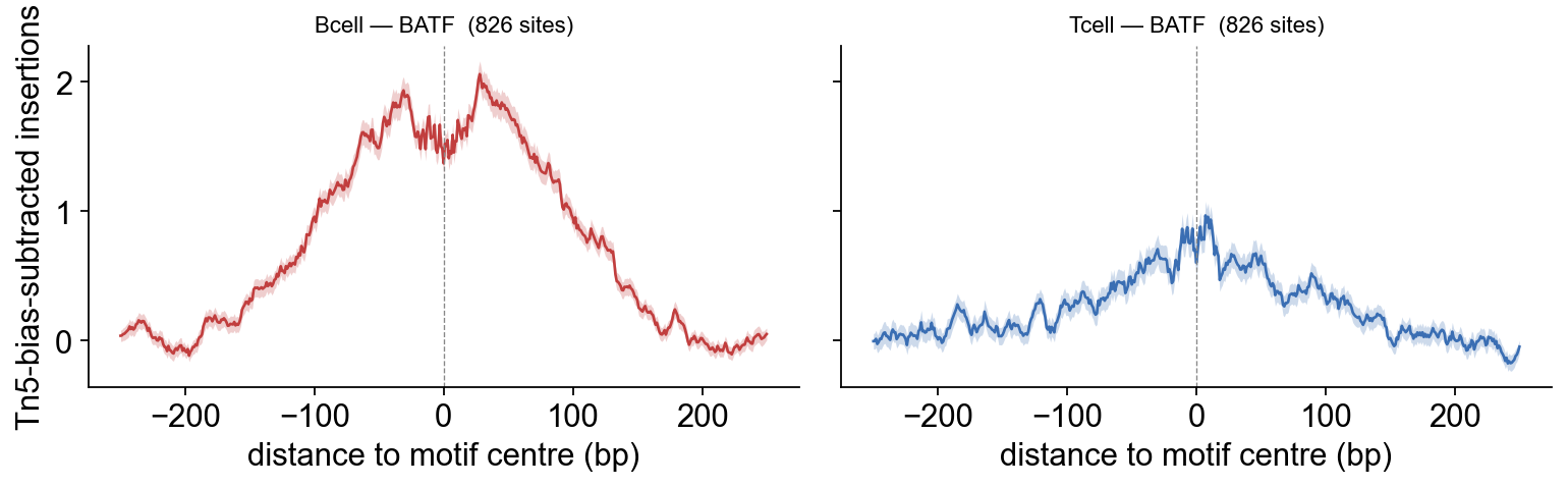
The biology recovers the same way in both backends: on this chr4 subset BATF shows a deeper footprint in Bcell than Tcell. More importantly, the TOBIAS plot_aggregate (§2.7) and the ArchR overlay (§3.5) agree on which sample wins — exactly the cross-backend consistency this tutorial is built around.

4 · Choosing between backends

Question	Backend
Two (or more) ATAC conditions — I want TFs whose binding differs, with p-values	TOBIAS → atacorrect → score_bigwig → bindetect
One or more samples — I want a clean per-TF footprint plot	ArchR → footprint_archr → plot_footprints
I need corrected signal as a bigwig for genome-browser inspection	TOBIAS (atacorrect writes one directly)
I already use epione for scATAC and want bulk and single-cell footprints to share the algorithm	ArchR (reuses epi.tl.get_footprints)