Upstream tutorial: CUT&RUN

Upstream tutorial: CUT&RUN#

This notebook is an epione-native adaptation of the Galaxy Training Network CUT&RUN tutorial. The overall aim is to start from paired-end FASTQ files, preprocess each replicate, merge them into an experiment-level BAM, generate a bigWig signal track, call peaks, and then inspect whether the resulting signal behaves as expected at both a representative locus and around transcription start sites.

The Galaxy lesson teaches this as a browser-based workflow made of multiple tool invocations. Here we keep the same conceptual sequence, but express the workflow as a compact set of epi.upstream.* calls so that the notebook doubles as a reusable pipeline prototype for the OTX2 project.

As in the ATAC notebook, the example is deliberately engineered to be executable. We therefore use the small public GTN teaching FASTQs and a lightweight chr22 reference derived from a local GRCh38 cache. That allows the full workflow to run in omicdev while preserving the important CUT&RUN ideas: replicate-aware preprocessing, merged coverage generation, peak calling, browser-style signal inspection, and promoter-centred aggregation.

Scope note. This notebook focuses on the upstream path of a bulk CUT&RUN analysis: FASTQ -> per-replicate BAM -> merged BAM -> bigWig -> peaks -> visual QC. It does not attempt to cover full replicate concordance statistics, motif analysis, or downstream comparative biology.

Data provenance#

The example inputs are the small replicate FASTQs distributed with the Galaxy Training Network CUT&RUN tutorial. They are designed for teaching, but they preserve an important real-world property that many toy datasets omit: a two-replicate structure that has to be processed and then merged.

Item	Source	How it is used here
Rep1 / Rep2 paired-end FASTQs	Galaxy GTN CUT&RUN tutorial toy dataset	Demonstrate replicate-level preprocessing and experiment-level merging.
GRCh38 FASTA	Local cache on this machine	Used to derive a small executable `chr22` reference.
Merged peak locus	Chosen from the strongest MACS2 peak in the merged demo run	Used for a compact browser-style quality check.

Local paths used throughout the notebook:

case/otx2/galaxy_cutrun_demo/
  fastq/     # downloaded GTN toy FASTQs
  ref/       # chr22 FASTA + bowtie2 index + derived annotation
  result/    # replicate BAMs, merged BAM, bigWigs, MACS2 peaks

Learning goals#

By the end of the notebook, you should be able to answer five practical questions:

How does epione represent the replicate-aware structure of a CUT&RUN preprocessing run?
Which part of the workflow is per-replicate, and which part is experiment-level?
How do we convert merged alignments into both a signal track and a peak set?
What does a reasonable merged CUT&RUN peak look like in a local browser plot?
How can the same compact API be transferred to the real OTX2 CUT&RUN samples?

import os
import pathlib
import urllib.request
import warnings

import pandas as pd
import epione as epi

warnings.filterwarnings('ignore', message='Function .* is missing a docstring.*')
os.environ['LC_ALL'] = 'C'
os.environ['LC_CTYPE'] = 'C'

epi.pl.plot_set()

WORK = pathlib.Path.cwd()
DATA = WORK / 'galaxy_cutrun_demo'
FASTQ_DIR = DATA / 'fastq'
REF_DIR = DATA / 'ref'
OUT = DATA / 'result'
for p in [FASTQ_DIR, REF_DIR, OUT]:
    p.mkdir(parents=True, exist_ok=True)

HG38_FASTA = pathlib.Path('/scratch/users/steorra/data/snapatac2_cache/gencode_v41_GRCh38.fa.gz.decomp')
CHR22_FASTA = REF_DIR / 'chr22.fa'
CHR22_BT2_PREFIX = REF_DIR / 'chr22'
CHR22_SIZE = 50818468

CUTRUN_URLS = {
    'Rep1_R1.fastq': 'https://zenodo.org/record/6823059/files/Rep1_R1.fastq',
    'Rep1_R2.fastq': 'https://zenodo.org/record/6823059/files/Rep1_R2.fastq',
    'Rep2_R1.fastq': 'https://zenodo.org/record/6823059/files/Rep2_R1.fastq',
    'Rep2_R2.fastq': 'https://zenodo.org/record/6823059/files/Rep2_R2.fastq',
}

└─ 🔬 Starting plot initialization...
  ├─ Apply Scanpy/matplotlib settings
  ├─ Custom font setup
  ├─ Suppress warnings
  ├─ 
___________      .__                      
\_   _____/_____ |__| ____   ____   ____  
 |    __)_\____ \|  |/  _ \ /    \_/ __ \ 
 |        \  |_> >  (  <_> )   |  \  ___/ 
/_______  /   __/|__|\____/|___|  /\___  >
        \/|__|                  \/     \/ 

  ├─ 🔖 Version: 0.0.1rc1   📚 Tutorials: https://epione.readthedocs.io/
└─ ✅ plot_set complete.

1. Check upstream tools#

Even in a notebook-driven epione workflow, CUT&RUN preprocessing still depends on the usual alignment and BAM-processing ecosystem. The Galaxy tutorial hides that complexity behind separate tool forms; here we surface it explicitly before the first compute-heavy step.

The dependency check matters for two reasons. First, it makes the notebook more robust to reruns in a shared environment. Second, it clarifies which steps are genuinely handled by epione logic and which still rely on established external bioinformatics tools.

Tool family	Why it matters
`bowtie2`	Aligns paired-end CUT&RUN reads to the reference.
`samtools`	Sorts, filters, merges, and indexes BAM files.
`bedtools`	Supports interval-aware BAM-to-region conversions.
`MACS2`	Calls peaks from the merged alignment.
`epione` built-in bigWig writer	Default route for exporting normalized bigWig signal inside the Python workflow.

A short environment check is therefore not boilerplate. It is the fastest way to catch missing external dependencies before replicate processing starts.

epi.upstream.check_tools([
    'bowtie2',
    'samtools',
    'bedtools',
    'macs2',
])

✓  bowtie2                    /scratch/users/steorra/env/omicdev/bin/bowtie2
  ✓  samtools                   /scratch/users/steorra/env/omicdev/bin/samtools
  ✓  bedtools                   /scratch/users/steorra/env/omicdev/bin/bedtools
  ✓  macs2                      /scratch/users/steorra/env/omicdev/bin/macs2

{'bowtie2': '/scratch/users/steorra/env/omicdev/bin/bowtie2',
 'samtools': '/scratch/users/steorra/env/omicdev/bin/samtools',
 'bedtools': '/scratch/users/steorra/env/omicdev/bin/bedtools',
 'macs2': '/scratch/users/steorra/env/omicdev/bin/macs2'}

2. Download the Galaxy toy FASTQs#

The input files are the two replicate pairs from the Galaxy GTN CUT&RUN tutorial. These FASTQs are intentionally compact, but unlike many toy datasets they still preserve the replicate structure that matters for a realistic CUT&RUN workflow.

That design is useful pedagogically because it lets the notebook teach two layers of reasoning at once:

replicate-level preprocessing, where each pair is aligned and filtered independently, and
experiment-level summarisation, where the processed replicates are merged into a combined signal and peak set.

At this stage the notebook is simply establishing the raw inputs. Once the four FASTQs are present, the remaining steps can be expressed entirely through epi.upstream.* functions without any Galaxy-style dataset collection management.

for name, url in CUTRUN_URLS.items():
    out = FASTQ_DIR / name
    if not out.exists():
        print(f'downloading {name} ...')
        urllib.request.urlretrieve(url, out)
    else:
        print(f'skip existing: {name}')

pairs = [
    ('Rep1', FASTQ_DIR / 'Rep1_R1.fastq', FASTQ_DIR / 'Rep1_R2.fastq'),
    ('Rep2', FASTQ_DIR / 'Rep2_R1.fastq', FASTQ_DIR / 'Rep2_R2.fastq'),
]
pd.DataFrame({
    'sample': [s for s, _, _ in pairs],
    'fq1': [str(r1) for _, r1, _ in pairs],
    'fq2': [str(r2) for _, _, r2 in pairs],
})

downloading Rep1_R1.fastq ...
downloading Rep1_R2.fastq ...
downloading Rep2_R1.fastq ...
downloading Rep2_R2.fastq ...

	sample	fq1	fq2
0	Rep1	/scratch/users/steorra/analysis/omicverse_dev/...	/scratch/users/steorra/analysis/omicverse_dev/...
1	Rep2	/scratch/users/steorra/analysis/omicverse_dev/...	/scratch/users/steorra/analysis/omicverse_dev/...

3. Prepare a `chr22` demo reference#

As in the ATAC tutorial, the full human reference would be unnecessary overhead for a notebook whose purpose is to demonstrate workflow structure rather than produce publication-scale outputs. We therefore derive a small chr22 reference from a locally cached GRCh38 FASTA.

This reduced reference keeps the executable example aligned with the constraints of the local environment while still supporting the essential CUT&RUN operations: alignment, replicate processing, merging, coverage export, peak calling, and signal aggregation.

epi.upstream.prepare_reference(...) centralizes a step that often ends up scattered across shell commands. The point is not only convenience. It also guarantees that later epione calls are all reading from the same reference bundle rather than relying on loosely coordinated index files on disk.

%%time
from pyfaidx import Fasta

if not CHR22_FASTA.exists():
    fa = Fasta(str(HG38_FASTA))
    with open(CHR22_FASTA, 'w') as fout:
        fout.write('>chr22\n')
        seq = str(fa['chr22'])
        for i in range(0, len(seq), 60):
            fout.write(seq[i:i+60] + '\n')

ref = epi.upstream.prepare_reference(
    fasta=CHR22_FASTA,
    aligner='bowtie2',
    index_prefix=CHR22_BT2_PREFIX,
)
ref

Settings:
  Output files: "/scratch/users/steorra/analysis/omicverse_dev/epione/epione_guide/tutorials/bulk/galaxy_cutrun_demo/ref/chr22.*.bt2"
  Line rate: 6 (line is 64 bytes)
  Lines per side: 1 (side is 64 bytes)
  Offset rate: 4 (one in 16)
  FTable chars: 10
  Strings: unpacked
  Max bucket size: default
  Max bucket size, sqrt multiplier: default
  Max bucket size, len divisor: 4
  Difference-cover sample period: 1024
  Endianness: little
  Actual local endianness: little
  Sanity checking: disabled
  Assertions: disabled
  Random seed: 0
  Sizeofs: void*:8, int:4, long:8, size_t:8
Input files DNA, FASTA:
  /scratch/users/steorra/analysis/omicverse_dev/epione/epione_guide/tutorials/bulk/galaxy_cutrun_demo/ref/chr22.fa
Reading reference sizes
  Time reading reference sizes: 00:00:01
Calculating joined length
Writing header
Reserving space for joined string
Joining reference sequences
Time to join reference sequences: 00:00:00
bmax according to bmaxDivN setting: 9789944
Using parameters --bmax 7342458 --dcv 1024
  Doing ahead-of-time memory usage test
  Passed!  Constructing with these parameters: --bmax 7342458 --dcv 1024
Constructing suffix-array element generator
Building DifferenceCoverSample
  Building sPrime
  Building sPrimeOrder
  V-Sorting samples
V-Sorting samples time: 00:00:00
  Allocating rank array
  Ranking v-sort output
  Ranking v-sort output time: 00:00:00
  Invoking Larsson-Sadakane on ranks
Invoking Larsson-Sadakane on ranks time: 00:00:00
  Sanity-checking and returning
Building samples
Reserving space for 12 sample suffixes
Generating random suffixes
QSorting 12 sample offsets, eliminating duplicates
QSorting sample offsets, eliminating duplicates time: 00:00:00
Multikey QSorting 12 samples
  (Using difference cover)
  Multikey QSorting samples time: 00:00:00
Calculating bucket sizes
Splitting and merging
  Splitting and merging time: 00:00:00
Avg bucket size: 4.89497e+06 (target: 7342457)
Converting suffix-array elements to index image
Allocating ftab, absorbFtab
Entering Ebwt loop
Getting block 1 of 8
  Reserving size (7342458) for bucket 1
  Calculating Z arrays for bucket 1
  Entering block accumulator loop for bucket 1:
  bucket 1: 10%
  bucket 1: 20%
  bucket 1: 30%
  bucket 1: 40%
  bucket 1: 50%
bucket 1: 60%
  bucket 1: 70%
  bucket 1: 80%
  bucket 1: 90%
  bucket 1: 100%
  Sorting block of length 6109124 for bucket 1
  (Using difference cover)
Sorting block time: 00:00:01
Returning block of 6109125 for bucket 1
Getting block 2 of 8
  Reserving size (7342458) for bucket 2
  Calculating Z arrays for bucket 2
  Entering block accumulator loop for bucket 2:
  bucket 2: 10%
  bucket 2: 20%
  bucket 2: 30%
  bucket 2: 40%
bucket 2: 50%
  bucket 2: 60%
  bucket 2: 70%
  bucket 2: 80%
  bucket 2: 90%
bucket 2: 100%
  Sorting block of length 4162165 for bucket 2
  (Using difference cover)
Sorting block time: 00:00:01
Returning block of 4162166 for bucket 2
Getting block 3 of 8
  Reserving size (7342458) for bucket 3
  Calculating Z arrays for bucket 3
  Entering block accumulator loop for bucket 3:
  bucket 3: 10%
bucket 3: 20%
  bucket 3: 30%
  bucket 3: 40%
  bucket 3: 50%
  bucket 3: 60%
bucket 3: 70%
  bucket 3: 80%
  bucket 3: 90%
  bucket 3: 100%
  Sorting block of length 3242487 for bucket 3
  (Using difference cover)
Sorting block time: 00:00:01
Returning block of 3242488 for bucket 3
Getting block 4 of 8
  Reserving size (7342458) for bucket 4
  Calculating Z arrays for bucket 4
  Entering block accumulator loop for bucket 4:
  bucket 4: 10%
bucket 4: 20%
  bucket 4: 30%
  bucket 4: 40%
  bucket 4: 50%
bucket 4: 60%
  bucket 4: 70%
  bucket 4: 80%
  bucket 4: 90%
bucket 4: 100%
  Sorting block of length 5059508 for bucket 4
  (Using difference cover)
Sorting block time: 00:00:01
Returning block of 5059509 for bucket 4
Getting block 5 of 8
  Reserving size (7342458) for bucket 5
  Calculating Z arrays for bucket 5
  Entering block accumulator loop for bucket 5:
bucket 5: 10%
  bucket 5: 20%
  bucket 5: 30%
  bucket 5: 40%
bucket 5: 50%
  bucket 5: 60%
  bucket 5: 70%
  bucket 5: 80%
bucket 5: 90%
  bucket 5: 100%
  Sorting block of length 2717729 for bucket 5
  (Using difference cover)
Sorting block time: 00:00:00
Returning block of 2717730 for bucket 5
Getting block 6 of 8
  Reserving size (7342458) for bucket 6
  Calculating Z arrays for bucket 6
  Entering block accumulator loop for bucket 6:
  bucket 6: 10%
  bucket 6: 20%
bucket 6: 30%
  bucket 6: 40%
  bucket 6: 50%
  bucket 6: 60%
bucket 6: 70%
  bucket 6: 80%
  bucket 6: 90%
  bucket 6: 100%
  Sorting block of length 6052533 for bucket 6
  (Using difference cover)
Sorting block time: 00:00:01
Returning block of 6052534 for bucket 6
Getting block 7 of 8
  Reserving size (7342458) for bucket 7
  Calculating Z arrays for bucket 7
  Entering block accumulator loop for bucket 7:
  bucket 7: 10%
  bucket 7: 20%
  bucket 7: 30%
bucket 7: 40%
  bucket 7: 50%
  bucket 7: 60%
  bucket 7: 70%
bucket 7: 80%
  bucket 7: 90%
  bucket 7: 100%
  Sorting block of length 6696876 for bucket 7
  (Using difference cover)
Sorting block time: 00:00:05
Returning block of 6696877 for bucket 7
Getting block 8 of 8
  Reserving size (7342458) for bucket 8
  Calculating Z arrays for bucket 8
  Entering block accumulator loop for bucket 8:
  bucket 8: 10%
  bucket 8: 20%
  bucket 8: 30%
bucket 8: 40%
  bucket 8: 50%
  bucket 8: 60%
  bucket 8: 70%
  bucket 8: 80%
bucket 8: 90%
  bucket 8: 100%
  Sorting block of length 5119348 for bucket 8
  (Using difference cover)
Sorting block time: 00:00:02
Returning block of 5119349 for bucket 8
Exited Ebwt loop
fchr[A]: 0
fchr[C]: 10382214
fchr[G]: 19542866
fchr[T]: 28789052
fchr[$]: 39159777
Exiting Ebwt::buildToDisk()
Returning from initFromVector
Wrote 17248347 bytes to primary EBWT file: /scratch/users/steorra/analysis/omicverse_dev/epione/epione_guide/tutorials/bulk/galaxy_cutrun_demo/ref/chr22.1.bt2.tmp
Wrote 9789952 bytes to secondary EBWT file: /scratch/users/steorra/analysis/omicverse_dev/epione/epione_guide/tutorials/bulk/galaxy_cutrun_demo/ref/chr22.2.bt2.tmp
Re-opening _in1 and _in2 as input streams
Returning from Ebwt constructor
Headers:
    len: 39159777
    bwtLen: 39159778
    sz: 9789945
    bwtSz: 9789945
    lineRate: 6
    offRate: 4
    offMask: 0xfffffff0
    ftabChars: 10
    eftabLen: 20
    eftabSz: 80
    ftabLen: 1048577
    ftabSz: 4194308
    offsLen: 2447487
    offsSz: 9789948
    lineSz: 64
    sideSz: 64
    sideBwtSz: 48
    sideBwtLen: 192
    numSides: 203958
    numLines: 203958
    ebwtTotLen: 13053312
    ebwtTotSz: 13053312
    color: 0
    reverse: 0
Total time for call to driver() for forward index: 00:00:18
Reading reference sizes
  Time reading reference sizes: 00:00:00
Calculating joined length
Writing header
Reserving space for joined string
Joining reference sequences
Time to join reference sequences: 00:00:01
  Time to reverse reference sequence: 00:00:00
bmax according to bmaxDivN setting: 9789944
Using parameters --bmax 7342458 --dcv 1024
  Doing ahead-of-time memory usage test
  Passed!  Constructing with these parameters: --bmax 7342458 --dcv 1024
Constructing suffix-array element generator
Building DifferenceCoverSample
  Building sPrime
  Building sPrimeOrder
  V-Sorting samples
V-Sorting samples time: 00:00:00
  Allocating rank array
  Ranking v-sort output
  Ranking v-sort output time: 00:00:00
  Invoking Larsson-Sadakane on ranks
Invoking Larsson-Sadakane on ranks time: 00:00:00
  Sanity-checking and returning
Building samples
Reserving space for 12 sample suffixes
Generating random suffixes
QSorting 12 sample offsets, eliminating duplicates
QSorting sample offsets, eliminating duplicates time: 00:00:00
Multikey QSorting 12 samples
  (Using difference cover)
  Multikey QSorting samples time: 00:00:00
Calculating bucket sizes
Splitting and merging
  Splitting and merging time: 00:00:00
Avg bucket size: 5.59425e+06 (target: 7342457)
Converting suffix-array elements to index image
Allocating ftab, absorbFtab
Entering Ebwt loop
Getting block 1 of 7
  Reserving size (7342458) for bucket 1
  Calculating Z arrays for bucket 1
  Entering block accumulator loop for bucket 1:
  bucket 1: 10%
  bucket 1: 20%
  bucket 1: 30%
  bucket 1: 40%
  bucket 1: 50%
bucket 1: 60%
  bucket 1: 70%
  bucket 1: 80%
  bucket 1: 90%
  bucket 1: 100%
  Sorting block of length 6882572 for bucket 1
  (Using difference cover)
Sorting block time: 00:00:01
Returning block of 6882573 for bucket 1
Getting block 2 of 7
  Reserving size (7342458) for bucket 2
  Calculating Z arrays for bucket 2
  Entering block accumulator loop for bucket 2:
  bucket 2: 10%
  bucket 2: 20%
  bucket 2: 30%
bucket 2: 40%
  bucket 2: 50%
  bucket 2: 60%
  bucket 2: 70%
  bucket 2: 80%
bucket 2: 90%
  bucket 2: 100%
  Sorting block of length 7217801 for bucket 2
  (Using difference cover)
Sorting block time: 00:00:01
Returning block of 7217802 for bucket 2
Getting block 3 of 7
  Reserving size (7342458) for bucket 3
  Calculating Z arrays for bucket 3
  Entering block accumulator loop for bucket 3:
  bucket 3: 10%
  bucket 3: 20%
  bucket 3: 30%
bucket 3: 40%
  bucket 3: 50%
  bucket 3: 60%
  bucket 3: 70%
bucket 3: 80%
  bucket 3: 90%
  bucket 3: 100%
  Sorting block of length 6398765 for bucket 3
  (Using difference cover)
Sorting block time: 00:00:01
Returning block of 6398766 for bucket 3
Getting block 4 of 7
  Reserving size (7342458) for bucket 4
  Calculating Z arrays for bucket 4
  Entering block accumulator loop for bucket 4:
  bucket 4: 10%
  bucket 4: 20%
  bucket 4: 30%
bucket 4: 40%
  bucket 4: 50%
  bucket 4: 60%
  bucket 4: 70%
bucket 4: 80%
  bucket 4: 90%
  bucket 4: 100%
  Sorting block of length 2716193 for bucket 4
  (Using difference cover)
Sorting block time: 00:00:00
Returning block of 2716194 for bucket 4
Getting block 5 of 7
  Reserving size (7342458) for bucket 5
  Calculating Z arrays for bucket 5
  Entering block accumulator loop for bucket 5:
  bucket 5: 10%
bucket 5: 20%
  bucket 5: 30%
  bucket 5: 40%
  bucket 5: 50%
bucket 5: 60%
  bucket 5: 70%
  bucket 5: 80%
  bucket 5: 90%
  bucket 5: 100%
  Sorting block of length 5106643 for bucket 5
  (Using difference cover)
Sorting block time: 00:00:00
Returning block of 5106644 for bucket 5
Getting block 6 of 7
  Reserving size (7342458) for bucket 6
  Calculating Z arrays for bucket 6
  Entering block accumulator loop for bucket 6:
bucket 6: 10%
  bucket 6: 20%
  bucket 6: 30%
  bucket 6: 40%
bucket 6: 50%
  bucket 6: 60%
  bucket 6: 70%
  bucket 6: 80%
bucket 6: 90%
  bucket 6: 100%
  Sorting block of length 6895232 for bucket 6
  (Using difference cover)
Sorting block time: 00:00:01
Returning block of 6895233 for bucket 6
Getting block 7 of 7
  Reserving size (7342458) for bucket 7
  Calculating Z arrays for bucket 7
  Entering block accumulator loop for bucket 7:
  bucket 7: 10%
  bucket 7: 20%
  bucket 7: 30%
  bucket 7: 40%
  bucket 7: 50%
  bucket 7: 60%
bucket 7: 70%
  bucket 7: 80%
  bucket 7: 90%
  bucket 7: 100%
  Sorting block of length 3942565 for bucket 7
  (Using difference cover)
Sorting block time: 00:00:01
Returning block of 3942566 for bucket 7
Exited Ebwt loop
fchr[A]: 0
fchr[C]: 10382214
fchr[G]: 19542866
fchr[T]: 28789052
fchr[$]: 39159777
Exiting Ebwt::buildToDisk()
Returning from initFromVector
Wrote 17248347 bytes to primary EBWT file: /scratch/users/steorra/analysis/omicverse_dev/epione/epione_guide/tutorials/bulk/galaxy_cutrun_demo/ref/chr22.rev.1.bt2.tmp
Wrote 9789952 bytes to secondary EBWT file: /scratch/users/steorra/analysis/omicverse_dev/epione/epione_guide/tutorials/bulk/galaxy_cutrun_demo/ref/chr22.rev.2.bt2.tmp
Re-opening _in1 and _in2 as input streams
Returning from Ebwt constructor
Headers:
    len: 39159777
    bwtLen: 39159778
    sz: 9789945
    bwtSz: 9789945
    lineRate: 6
    offRate: 4
    offMask: 0xfffffff0
    ftabChars: 10
    eftabLen: 20
    eftabSz: 80
    ftabLen: 1048577
    ftabSz: 4194308
    offsLen: 2447487
    offsSz: 9789948
    lineSz: 64
    sideSz: 64
    sideBwtSz: 48
    sideBwtLen: 192
    numSides: 203958
    numLines: 203958
    ebwtTotLen: 13053312
    ebwtTotSz: 13053312
    color: 0
    reverse: 1
Total time for backward call to driver() for mirror index: 00:00:12
CPU times: user 219 ms, sys: 85.4 ms, total: 305 ms
Wall time: 30.2 s

{'fasta': '/scratch/users/steorra/analysis/omicverse_dev/epione/epione_guide/tutorials/bulk/galaxy_cutrun_demo/ref/chr22.fa',
 'fai': '/scratch/users/steorra/analysis/omicverse_dev/epione/epione_guide/tutorials/bulk/galaxy_cutrun_demo/ref/chr22.fa.fai',
 'chrom_sizes': '/scratch/users/steorra/analysis/omicverse_dev/epione/epione_guide/tutorials/bulk/galaxy_cutrun_demo/ref/chr22.chrom.sizes',
 'ref_index': '/scratch/users/steorra/analysis/omicverse_dev/epione/epione_guide/tutorials/bulk/galaxy_cutrun_demo/ref/chr22'}

4. Process each replicate step by step#

The Galaxy CUT&RUN lesson describes a sequence of trimming, alignment, filtering, duplicate removal, and coverage export. In epione we now represent that same logic explicitly instead of hiding it inside a single helper.

For each replicate we run:

epi.upstream.bowtie2.align_fastq_to_bam(...) to build the coordinate-sorted BAM.
epi.upstream.samtools.filter_bam(...) to define the retained alignment set.
epi.upstream.samtools.index_bam(...) so the filtered BAM can be reused directly.
epi.upstream.bigwig.bam_to_bigwig(...) to export the replicate signal track.

This makes the replicate structure very clear. Each replicate leaves behind its own filtered BAM and bigWig before any merge occurs.

%%time
cutrun_runs = {}
for sample_name, fq1, fq2 in pairs:
    sample_dir = OUT / sample_name
    sample_dir.mkdir(parents=True, exist_ok=True)
    raw_bam = sample_dir / f'{sample_name}.raw.bam'
    filt_bam = sample_dir / f'{sample_name}.filtered.bam'
    bw_path = sample_dir / f'{sample_name}.rpkm.bw'

    for stale in [raw_bam, filt_bam, pathlib.Path(str(filt_bam) + '.bai'), bw_path]:
        if stale.exists():
            stale.unlink()

    epi.upstream.bowtie2.align_fastq_to_bam(
        fq1=str(fq1),
        fq2=str(fq2),
        out_bam=raw_bam,
        ref_index=ref['ref_index'],
        threads=8,
        extra_args=[
            '--end-to-end', '--very-sensitive', '--no-mixed', '--no-discordant',
            '-I', '10', '-X', '700',
        ],
        remove_duplicates=True,
    )
    epi.upstream.samtools.filter_bam(
        raw_bam,
        filt_bam,
        mapq=30,
        proper_pair=True,
        drop_secondary_supp=True,
        drop_duplicates=False,
        drop_qcfail=False,
        drop_unmapped=True,
        drop_mate_unmapped=True,
        threads=8,
    )
    epi.upstream.samtools.index_bam(filt_bam, threads=8)
    epi.upstream.bigwig.bam_to_bigwig(
        filt_bam,
        bw_path,
        bin_size=100,
        normalize_using='RPKM',
        threads=8,
    )
    raw_bam.unlink(missing_ok=True)
    cutrun_runs[sample_name] = {'bam': str(filt_bam), 'bigwig': str(bw_path)}

pd.DataFrame(cutrun_runs).T

CPU times: user 5 s, sys: 117 ms, total: 5.12 s
Wall time: 11.9 s

	bam	bigwig
Rep1	/scratch/users/steorra/analysis/omicverse_dev/...	/scratch/users/steorra/analysis/omicverse_dev/...
Rep2	/scratch/users/steorra/analysis/omicverse_dev/...	/scratch/users/steorra/analysis/omicverse_dev/...

5. Merge replicate BAMs and export the experiment-level track#

Once both replicates have been processed individually, we switch from replicate-level reasoning to experiment-level summarisation.

Operation	`epione` function	Purpose
Merge filtered replicate BAMs	`epi.upstream.samtools.merge_bams(...)`	Produces one experiment-level alignment from the retained replicate reads.
Export merged coverage	`epi.upstream.bigwig.bam_to_bigwig(...)`	Creates the combined signal track used for visualization and matrix aggregation.

This keeps the provenance clean: replicate BAMs remain available, but the merged signal is what we inspect for the rest of the tutorial.

%%time
merged_dir = OUT / 'merged'
merged_dir.mkdir(parents=True, exist_ok=True)
for stale in [merged_dir / 'Rep12.filtered.bam', merged_dir / 'Rep12.filtered.bam.bai', merged_dir / 'Rep12.rpkm.bw']:
    if stale.exists():
        stale.unlink()

merged_bam = epi.upstream.samtools.merge_bams(
    [cutrun_runs['Rep1']['bam'], cutrun_runs['Rep2']['bam']],
    merged_dir / 'Rep12.filtered.bam',
    threads=8,
    index=True,
)
merged_bw = epi.upstream.bigwig.bam_to_bigwig(
    merged_bam,
    merged_dir / 'Rep12.rpkm.bw',
    bin_size=100,
    normalize_using='RPKM',
    threads=8,
)
{'merged_bam': merged_bam, 'merged_bigwig': merged_bw}

CPU times: user 2.49 s, sys: 55.7 ms, total: 2.55 s
Wall time: 2.6 s

{'merged_bam': '/scratch/users/steorra/analysis/omicverse_dev/epione/epione_guide/tutorials/bulk/galaxy_cutrun_demo/result/merged/Rep12.filtered.bam',
 'merged_bigwig': '/scratch/users/steorra/analysis/omicverse_dev/epione/epione_guide/tutorials/bulk/galaxy_cutrun_demo/result/merged/Rep12.rpkm.bw'}

6. Peak calling on the merged BAM#

After merging, the next goal is to summarize the strongest reproducible enrichment events as a standard peak set. In the Galaxy tutorial, this step comes after mapping and filtering once the signal is judged clean enough to support interval-level interpretation.

The function#

epi.upstream.macs2.call_peaks_macs2(...) provides the thin epione wrapper around MACS2 peak calling.

Key parameter	What it controls
`bam`	The merged experiment-level alignment used as input signal.
`format='BAMPE'`	Uses paired-end fragment logic.
`qvalue`	Reporting threshold for significant peaks.
`call_summits=True`	Requests local summit positions inside peaks.
`nomodel=True`	Skips model building, which is often appropriate in CUT&RUN-like workflows.

Because the executable notebook uses a reduced chr22 reference, the emphasis is on producing a coherent tutorial output that can be interpreted visually rather than a definitive biological peak catalogue.

%%time
peak_paths = epi.upstream.macs2.call_peaks_macs2(
    bam=merged_bam,
    out_dir=OUT / 'peaks',
    name='Rep12',
    genome_size=str(CHR22_SIZE),
    format='BAMPE',
    qvalue=0.01,
    keep_dup='all',
    call_summits=True,
    nomodel=True,
)
peak_paths

CPU times: user 847 μs, sys: 897 μs, total: 1.74 ms
Wall time: 212 ms

{'narrowPeak': '/scratch/users/steorra/analysis/omicverse_dev/epione/epione_guide/tutorials/bulk/galaxy_cutrun_demo/result/peaks/Rep12_peaks.narrowPeak',
 'summits': '/scratch/users/steorra/analysis/omicverse_dev/epione/epione_guide/tutorials/bulk/galaxy_cutrun_demo/result/peaks/Rep12_summits.bed',
 'xls': '/scratch/users/steorra/analysis/omicverse_dev/epione/epione_guide/tutorials/bulk/galaxy_cutrun_demo/result/peaks/Rep12_peaks.xls'}

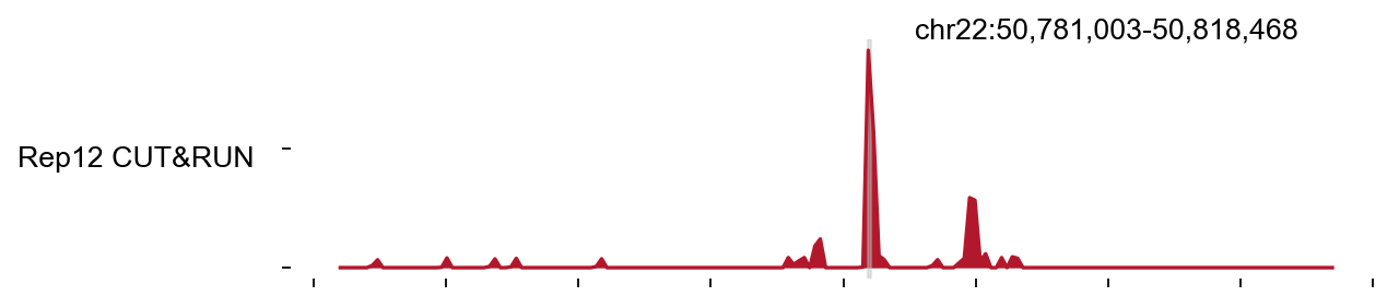
7. Visualise the strongest merged CUT&RUN peak#

A peak file is useful, but it is still a summary object. The next step is to verify that at least one representative peak is visually supported by a clear local enrichment profile in the merged bigWig. This mirrors the logic of the Galaxy tutorial, which spends substantial effort on interpreting coverage rather than treating the peak caller as infallible.

Biological question#

Does the top merged peak correspond to a sharp, localized coverage enrichment in the merged CUT&RUN track?

The function#

epi.bulk.bigwig(...).plot_track(...) renders the merged bigWig as a browser-style track around a chosen genomic window.

Key parameter	What it controls
`chrom`, `chromstart`, `chromend`	The local genomic window to display.
`plot_names`	Which registered bigWig tracks are shown.
`bp_per_bin`	Horizontal aggregation resolution.
`region_dict`	Highlight intervals, here the top merged peak.
`color_dict`	Per-track visual styling.

How to read the plot#

The key consistency check is simple: the highlighted peak interval should sit on top of a visibly enriched signal profile rather than a flat or noisy background. That does not prove biological correctness on its own, but it is one of the fastest local sanity checks for a compact CUT&RUN demo.

peak_df = pd.read_csv(peak_paths['narrowPeak'], sep='	', header=None)
top_peak = peak_df.sort_values(6, ascending=False).iloc[0]
chrom = str(top_peak[0])
center = int((int(top_peak[1]) + int(top_peak[2])) / 2)

bw_obj = epi.bulk.bigwig({'Rep12 CUT&RUN': merged_bw})
bw_obj.read()
chrom_len = bw_obj.bw_dict['Rep12 CUT&RUN'].chroms()[chrom]
start = max(0, center - 20000)
end = min(int(chrom_len), center + 20000)
region_dict = {'top_peak': (int(top_peak[1]), int(top_peak[2]))}
color_dict = {'Rep12 CUT&RUN': '#B2182B'}

bw_obj.plot_track(
    chrom=chrom,
    chromstart=start,
    chromend=end,
    plot_names=['Rep12 CUT&RUN'],
    figwidth=8,
    figheight=1.8,
    color_dict=color_dict,
    bp_per_bin=200,
    region_dict=region_dict,
)

└─ Load bigWig files
  └─ Loading Rep12 CUT&RUN...

(<Figure size 640x144 with 1 Axes>, [<Axes: ylabel='Rep12 CUT&RUN'>])

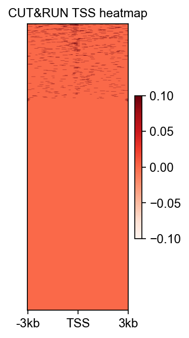
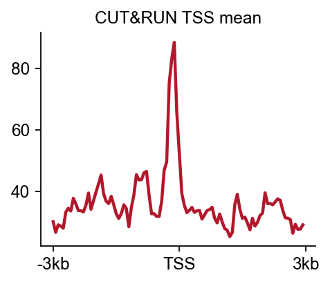
../../_images/c159692eb0ebc01e0dd8ab1fb22fb8a4265bc957f2c82c00b646605e4d5fc960.png

8. Compute a TSS heatmap with `epi.bulk.bigwig`#

The local browser view above answers a single-locus question. To add a more global summary, we also compute a TSS-centred signal matrix and render it as a heatmap plus a mean profile. This plays the same pedagogical role as the matrix-aggregation steps commonly shown in Galaxy tutorials.

Biological question#

When the merged CUT&RUN bigWig is summarized around annotated transcription start sites, does it show structured promoter-proximal signal rather than an undifferentiated background profile?

Why derive a small `chr22` GTF?#

The notebook uses a reduced chr22 reference, so the annotation has to match that reduced coordinate system. Rather than shipping a separate annotation file just for the tutorial, we derive a minimal transcript-only GTF from the local GRCh38 GENCODE gff3.

The functions#

This section uses the same matrix workflow taught elsewhere in epione:

load_gtf(...) registers transcript coordinates.
compute_matrix(...) aggregates signal around TSSs.
plot_matrix(...) visualizes the per-gene matrix.
plot_matrix_line(...) shows the average TSS profile.

Output	Interpretation
Heatmap	Whether promoter-proximal enrichment is broadly present across genes.
Mean profile	Whether signal is centered near the TSS rather than uniformly flat.

Together, the locus plot and the TSS matrix provide a local-plus-global view of the merged CUT&RUN signal quality.

GENCODE_GFF3 = pathlib.Path('/scratch/users/steorra/data/snapatac2_cache/gencode_v41_GRCh38.gff3.gz')
CHR22_GTF = REF_DIR / 'gencode_v41_chr22.transcripts.gtf'

CHR22_GTF = pathlib.Path(
    epi.utils.convert_gff_to_gtf(
        GENCODE_GFF3,
        CHR22_GTF,
        feature_whitelist=['transcript'],
        seqname_whitelist=['chr22'],
    )
)

with open(CHR22_GTF) as fin:
    transcript_count = sum(1 for _ in fin)

print(CHR22_GTF, transcript_count)

└─ Converting GFF to GTF: /scratch/users/steorra/data/snapatac2_cache/gencode_v41_GRCh38.gff3.gz -> /scratch/users/steorra/analysis/omicverse_dev/epione/epione_guide/tutorials/bulk/galaxy_cutrun_demo/ref/gencode_v41_chr22.transcripts.gtf
└─ Wrote 3939 GTF records
/scratch/users/steorra/analysis/omicverse_dev/epione/epione_guide/tutorials/bulk/galaxy_cutrun_demo/ref/gencode_v41_chr22.transcripts.gtf 3939

cutrun_tss = epi.bulk.bigwig({'Rep12 CUT&RUN': merged_bw})
cutrun_tss.read()
cutrun_tss.load_gtf(str(CHR22_GTF))
cutrun_tss.compute_matrix('Rep12 CUT&RUN', nbins=100, upstream=3000, downstream=3000, n_jobs=1)

fig, ax = cutrun_tss.plot_matrix(
    bw_name='Rep12 CUT&RUN',
    bw_type='TSS',
    figsize=(2.4, 4.2),
    cmap='Reds',
    vmax='auto',
    vmin='auto',
    fontsize=11,
    title='CUT&RUN TSS heatmap',
)

cutrun_tss.plot_matrix_line(
    bw_name='Rep12 CUT&RUN',
    bw_type='TSS',
    figsize=(3.2, 2.6),
    color='#B2182B',
    fontsize=11,
    title='CUT&RUN TSS mean',
)

└─ Load bigWig files
  └─ Loading Rep12 CUT&RUN...
└─ Load GTF file
  ├─ Reading GTF...
  └─ Reading GTF file from /scratch/users/steorra/analysis/omicverse_dev/epione/epione_guide/tutorials/bulk/galaxy_cutrun_demo/ref/gencode_v41_chr22.transcripts.gtf...
  └─ GTF file read successfully
  └─ GTF loaded
└─ Compute matrix: Rep12 CUT&RUN
  ├─ Prepare features
  ├─ Build matrices
└─ Finalize
  └─ Rep12 CUT&RUN matrix finished
  └─ Rep12 CUT&RUN tss matrix in bw_tss_scores_dict[Rep12 CUT&RUN]
  └─ Rep12 CUT&RUN tes matrix in bw_tes_scores_dict[Rep12 CUT&RUN]
  └─ Rep12 CUT&RUN body matrix in bw_body_scores_dict[Rep12 CUT&RUN]

(<Figure size 256x208 with 1 Axes>,
 <Axes: title={'center': 'CUT&RUN TSS mean'}>)

../../_images/1fb1c1803c22adfc4439e49b59858bbc785ba8e8f8d94f5ab18c205e2519a5cd.png

../../_images/9137bbc09f7bf58a3a7f93488047f17f9ff7063473aba4153a0fec5bad68765a.png

9. OTX2 project template#

The final code cell is the bridge from tutorial data to project data. It keeps the same explicit epi.upstream.bowtie2 -> epi.upstream.samtools -> epi.upstream.bigwig -> epi.upstream.macs2 structure used above, but swaps the GTN FASTQs for the real OTX2 CUT&RUN inputs.

That is the main advantage of rewriting the workflow this way: the teaching notebook and the production notebook share the same step-by-step API rather than a notebook-only convenience wrapper.

# rep1_dir = WORK / 'otx2_upstream' / 'cutrun_rep1'
# rep2_dir = WORK / 'otx2_upstream' / 'cutrun_rep2'
# rep1_dir.mkdir(parents=True, exist_ok=True)
# rep2_dir.mkdir(parents=True, exist_ok=True)
#
# rep1_raw = rep1_dir / 'h_OTX2_day2_CUTRUN_rep1.raw.bam'
# rep1_bam = rep1_dir / 'h_OTX2_day2_CUTRUN_rep1.filtered.bam'
# rep1_bw = rep1_dir / 'h_OTX2_day2_CUTRUN_rep1.rpkm.bw'
# rep2_raw = rep2_dir / 'h_OTX2_day2_CUTRUN_rep2.raw.bam'
# rep2_bam = rep2_dir / 'h_OTX2_day2_CUTRUN_rep2.filtered.bam'
# rep2_bw = rep2_dir / 'h_OTX2_day2_CUTRUN_rep2.rpkm.bw'
#
# epi.upstream.bowtie2.align_fastq_to_bam(
#     fq1='/path/to/h_OTX2_day2_CUTRUN_rep1_R1.fastq.gz',
#     fq2='/path/to/h_OTX2_day2_CUTRUN_rep1_R2.fastq.gz',
#     out_bam=rep1_raw,
#     ref_index='/path/to/full/genome/index/prefix',
#     threads=8,
#     extra_args=['--end-to-end', '--very-sensitive', '--no-mixed', '--no-discordant', '-I', '10', '-X', '700'],
#     remove_duplicates=True,
# )
# epi.upstream.samtools.filter_bam(rep1_raw, rep1_bam, mapq=30, proper_pair=True, drop_secondary_supp=True, drop_unmapped=True, drop_mate_unmapped=True, threads=8)
# epi.upstream.samtools.index_bam(rep1_bam, threads=8)
# epi.upstream.bigwig.bam_to_bigwig(rep1_bam, rep1_bw, bin_size=100, normalize_using='RPKM', threads=8)
#
# epi.upstream.bowtie2.align_fastq_to_bam(
#     fq1='/path/to/h_OTX2_day2_CUTRUN_rep2_R1.fastq.gz',
#     fq2='/path/to/h_OTX2_day2_CUTRUN_rep2_R2.fastq.gz',
#     out_bam=rep2_raw,
#     ref_index='/path/to/full/genome/index/prefix',
#     threads=8,
#     extra_args=['--end-to-end', '--very-sensitive', '--no-mixed', '--no-discordant', '-I', '10', '-X', '700'],
#     remove_duplicates=True,
# )
# epi.upstream.samtools.filter_bam(rep2_raw, rep2_bam, mapq=30, proper_pair=True, drop_secondary_supp=True, drop_unmapped=True, drop_mate_unmapped=True, threads=8)
# epi.upstream.samtools.index_bam(rep2_bam, threads=8)
# epi.upstream.bigwig.bam_to_bigwig(rep2_bam, rep2_bw, bin_size=100, normalize_using='RPKM', threads=8)
#
# rep12_bam = epi.upstream.samtools.merge_bams([rep1_bam, rep2_bam], WORK / 'otx2_upstream' / 'cutrun_rep12.bam', threads=8)
# peak_paths = epi.upstream.macs2.call_peaks_macs2(
#     bam=rep12_bam,
#     out_dir=WORK / 'otx2_upstream' / 'peaks',
#     name='h_OTX2_day2_CUTRUN',
#     genome_size='hs',
#     format='BAMPE',
#     qvalue=0.01,
#     keep_dup='all',
#     call_summits=True,
#     nomodel=True,
# )

Upstream tutorial: CUT&RUN

Contents

Upstream tutorial: CUT&RUN#

Data provenance#

Learning goals#

1. Check upstream tools#

2. Download the Galaxy toy FASTQs#

3. Prepare a chr22 demo reference#

4. Process each replicate step by step#

5. Merge replicate BAMs and export the experiment-level track#

6. Peak calling on the merged BAM#

The function#

7. Visualise the strongest merged CUT&RUN peak#

Biological question#

The function#

How to read the plot#

8. Compute a TSS heatmap with epi.bulk.bigwig#

Biological question#

Why derive a small chr22 GTF?#

The functions#

9. OTX2 project template#

3. Prepare a `chr22` demo reference#

8. Compute a TSS heatmap with `epi.bulk.bigwig`#

Why derive a small `chr22` GTF?#