Motif and TF activity with chromVAR

Motif and TF activity with chromVAR#

chromVAR (Schep et al., Nat Methods 2017) scores per-cell TF activity from a sparse scATAC-seq peak-by-cell matrix. For each motif and each cell it computes a bias-corrected Z-score that reflects how much more (or less) the cell’s reads pile up on peaks containing the motif than expected by chance. The score is bias-corrected because sequencing depth and GC content, not biology, otherwise dominate peak-level counts.

Epione provides the three-step chromVAR pipeline with ArchR-equivalent behaviour:

Step	Function	Produces
1	`epi.tl.add_motif_matrix`	`varm['motif']` — peak × motif binary matrix
2	`epi.tl.add_background_peaks`	`varm['bg_peaks']` — per-peak bias-matched peers
3	`epi.tl.compute_deviations`	`obsm['motif_deviations']` — cell × motif Z-scores

The default deviation estimator is method='analytical', a closed-form null that is ~10–40× faster than the original sample-based procedure and is the n_iter → ∞ limit of it. Pass method='sample' for bit-level chromVAR / ArchR reproducibility.

This tutorial walks through the pipeline on the public snapATAC2 pbmc5k dataset (≈5 k PBMCs × 50 k tile peaks) and reproduces ArchR’s three canonical chromVAR plots: TF variability, UMAP coloured by TF Z-score, and cluster × TF heatmap.

Part 1 · What chromVAR computes#

For a foreground motif $j$ and cell $c$:

Observed peak counts with motif $j$: $$\text{obs}_{j,c} = \sum_{i \in P_j} X_{i,c}$$ where $P_j$ is the set of peaks containing motif $j$ and $X_{i,c}$ is the count in peak $i$ of cell $c$.
Expected counts under the null (peak occupancy proportional to each peak’s global accessibility): $$\text{exp}_{j,c} = n_c \cdot \sum_{i \in P_j} p_i, \quad p_i = \tfrac{\sum_c X_{i,c}}{\sum_{i,c} X_{i,c}}$$ where $n_c$ is the per-cell total count.
Raw deviation: $$\text{dev}_{j,c} = \frac{\text{obs}_{j,c} - \text{exp}_{j,c}}{\text{exp}_{j,c}}$$
Bias correction. Each foreground peak is matched to $K$ peers with similar GC content and mean accessibility (the add_background_peaks step). For each of the $K$ background draws we substitute the peer peaks and recompute a deviation, then standardise: $$Z_{j,c} = \frac{\text{dev}_{j,c} - \text{mean}(\text{bg dev})_{j,c}}{\text{std}(\text{bg dev})_{j,c}}$$

The heavy lifting is step 4: repeating step 3 across n_iter background samples. Epione’s analytical estimator uses peak independence of the peer draws to collapse this into two sparse×dense matmuls — same biology, no Monte-Carlo noise.

Part 2 · Setup and load pbmc5k#

We use the public snapATAC2 pbmc5k fragment file, bin into 5 kb tiles, filter cells and select the top 50 k most-accessible tiles. If the intermediate AnnData is on disk we just reload it; otherwise the cell below runs the full import + QC in ~3 min.

import pathlib

import numpy as np
import pandas as pd
import anndata as ad
import anndataoom as oom
import scanpy as sc
import epione as epi

import matplotlib as mpl
import matplotlib.pyplot as plt
from IPython.display import display

epi.pl.plot_set()

WORK = pathlib.Path.cwd() / 'data_chromvar'
WORK.mkdir(parents=True, exist_ok=True)

└─ 🔬 Starting plot initialization...
  ├─ Apply Scanpy/matplotlib settings
  ├─ Custom font setup
  ├─ Suppress warnings
  ├─ 
___________      .__                      
\_   _____/_____ |__| ____   ____   ____  
 |    __)_\____ \|  |/  _ \ /    \_/ __ \ 
 |        \  |_> >  (  <_> )   |  \  ___/ 
/_______  /   __/|__|\____/|___|  /\___  >
        \/|__|                  \/     \/ 

  ├─ 🔖 Version: 0.0.1rc1   📚 Tutorials: https://epione.readthedocs.io/
└─ ✅ plot_set complete.

The snap.read / snap.pp.import_fragments call below is cached: once the pbmc5k.h5ad file exists it’s reloaded in milliseconds. The first run does fragment import + TSSe + cell filtering + 5 kb tile matrix construction + top-50 k feature selection.

%%time
# PBMC 5k ATAC — imports the 10x fragments file, computes QC and a
# 5 kb tile matrix. Cached to disk; re-runs in milliseconds.
h5 = WORK / 'pbmc5k.h5ad'
if h5.exists() and h5.stat().st_size > 100_000:
    data = oom.read(str(h5), backed='r+')
else:
    if h5.exists():
        h5.unlink()
    frag = epi.utils.register_datasets().fetch('atac_pbmc_5k.tsv.gz')
    data = epi.pp.import_fragments(
        str(frag),
        chrom_sizes=epi.utils.genome.hg38,
        file=str(h5),
        sorted_by_barcode=False,
    )
    genes = epi.utils.get_gene_annotation(epi.utils.genome.hg38)
    epi.pp.tsse(data, genes)
    data = epi.pp.filter_cells(data, min_counts=1000, max_counts=100000, min_tsse=5)
    epi.pp.add_tile_matrix(data, bin_size=5000)
    epi.pp.select_features(data, n_features=50000)
data

CPU times: user 1.02 s, sys: 1.06 s, total: 2.09 s
Wall time: 2.1 s

AnnDataOOM5,166obs×606,219varsRust · out-of-memory · backed

csr_matrix uint32 · 1.9% · ~87.3 MB/chunk · 674 MB disk · pbmc5k.h5ad

›obs4n_fragment · frac_dup · frac_mito · tsse

name	dtype	preview
`n_fragment`	uint64	22067, 10498, 19191, … (4657)
`frac_dup`	float64	0.5219143358537166, 0.5345186893096262, 0.5101962685995763, … (5165)
`frac_mito`	float64	0.0
`tsse`	float64	31.70564634504355, 29.54060864508625, 17.706611570247937, … (5027)

›var2count · selected

name	dtype	preview
`count`	float64	0.0, 15.0, 3.0, … (6370)
`selected`	bool	False, True

›obsm1fragment_paired

key	shape	dtype
`fragment_paired`	(5166, 3088286401)	uint32

›empty–varm · obsp · varp · layers · raw

Convert the snapATAC2 matrix + metadata into a plain AnnData. We keep only the tiles flagged as selected so downstream steps run on a ~50 k peak panel rather than the full ~600 k.

# ``epi.pp.add_tile_matrix`` writes a lazy anndataoom BackedArray;
# materialise it to a scipy.sparse.csr_matrix in memory so chromVAR
# can work with it like a plain AnnData.
from scipy import sparse
parts = []
for _, _, ch in data.X.chunked():
    parts.append(ch)
if sparse.issparse(parts[0]):
    X = sparse.vstack(parts).tocsr()
else:
    X = sparse.csr_matrix(np.vstack(parts))

obs = pd.DataFrame(data.obs).copy()
obs.index = list(data.obs_names)
var = pd.DataFrame(data.var).copy()
var.index = list(data.var_names)
adata = ad.AnnData(X=X, obs=obs, var=var)

# Restrict to the 50 k `selected` tiles — chromVAR runs on this peak panel.
if 'selected' in adata.var.columns:
    adata = adata[:, adata.var['selected'].astype(bool).values].copy()

print(f'adata: {adata.shape[0]:,} cells × {adata.shape[1]:,} peaks')
adata

adata: 5,166 cells × 50,000 peaks

AnnData object with n_obs × n_vars = 5166 × 50000
    obs: 'n_fragment', 'frac_dup', 'frac_mito', 'tsse'
    var: 'count', 'selected'

Part 3 · Cell embedding (for later plots)#

chromVAR itself doesn’t need clusters — the per-cell Z-scores are computed from the raw peak counts. But the downstream visualisations (UMAP coloured by TF Z-score, cluster × TF heatmap) need a 2-D embedding and cluster labels. epi.tl.iterative_lsi is ArchR-equivalent: two rounds of variable-feature TF-IDF + LSI, so the first LSI picks up gross structure and the second refines with within-cluster variable features. The result lives in obsm['X_iterative_lsi'].

%%time
# Two-iteration LSI (ArchR-style). Sample 5000 cells for the first-pass
# selection of variable features, then use all cells in iteration 2.
epi.tl.iterative_lsi(
    adata,
    n_components=30,
    iterations=2,
    var_features=10_000,
    resolution=0.5,
    n_neighbors=30,
    sample_cells_pre=5000,
    depth_col='n_fragment',
    seed=1,
)

# kNN graph on the LSI embedding, then Leiden clustering and UMAP.
sc.pp.neighbors(adata, use_rep='X_iterative_lsi', n_neighbors=30)
sc.tl.leiden(
    adata,
    resolution=0.5,
    flavor='igraph', directed=False, n_iterations=2,
    random_state=0, key_added='leiden',
)
sc.tl.umap(adata, random_state=0)

print(f"found {adata.obs['leiden'].nunique()} Leiden clusters")

└─ [iterative_lsi] Initial feature set: 49,755 / 50,000
└─ [iterative_lsi] Iter 1/2 | fit on 5,000 cells x 49,755 features
computing neighbors
finished: added to `.uns['neighbors']`
    `.obsp['distances']`, distances for each pair of neighbors
    `.obsp['connectivities']`, weighted adjacency matrix (0:00:35)
running Leiden clustering
finished: found 13 clusters and added
    'leiden', the cluster labels (adata.obs, categorical) (0:00:00)
└─ [iterative_lsi]   -> 13 clusters; selected 10,000 variable features for next round
└─ [iterative_lsi] Iter 2/2 | fit on 5,166 cells x 10,000 features
└─ [iterative_lsi] Done. Stored embedding (5,166 x 29) in adata.obsm['X_iterative_lsi']
computing neighbors
finished: added to `.uns['neighbors']`
    `.obsp['distances']`, distances for each pair of neighbors
    `.obsp['connectivities']`, weighted adjacency matrix (0:00:00)
running Leiden clustering
finished: found 8 clusters and added
    'leiden', the cluster labels (adata.obs, categorical) (0:00:00)
computing UMAP
finished: added
    'X_umap', UMAP coordinates (adata.obsm)
    'umap', UMAP parameters (adata.uns) (0:00:14)
found 8 Leiden clusters
CPU times: user 2min, sys: 3.86 s, total: 2min 3s
Wall time: 1min 11s

Part 4 · Motif annotation — peak × motif matrix#

For each (peak, motif) pair we need to know whether the motif’s position weight matrix (PWM) is present in the peak’s DNA sequence above a significance threshold. There are two ways to run this in Epione:

Direct mode — call MOODS on the peak sequences:

epi.tl.add_motif_matrix(
    adata,
    genome_fasta=str(snap.genome.hg38.fasta),
    motif_db='JASPAR2020',
    motif_tax_group=['vertebrates'],
    pvalue=5e-5,
)

This scans the ~50 k peaks against the ~750 JASPAR2020 CORE vertebrate motifs from scratch, which takes ~60–100 s per call.

Database mode (recommended) — pre-scan the whole genome once per (genome, motif collection, p-value) combination, then just look up hits that overlap the peak set:

epi.tl.build_motif_database(
    genome_fasta=str(snap.genome.hg38.fasta),
    out_dir='motif_db_hg38_jaspar2020_5e5',
    motif_db='JASPAR2020', motif_collection='CORE',
    motif_tax_group=['vertebrates'],
    p_value=5e-5, n_jobs=-1,
)

(Build takes ~3–6 min across 8 cores; the resulting parquet index is ~700 MB and is reusable across any dataset on the same reference.)

After that, annotation of new datasets drops to about a second:

%%time
# Point add_motif_matrix at the pre-built per-chromosome parquet index.
# For this tutorial we assume it lives in `motif_db_hg38_jaspar2020_5e5/`
# next to the notebook; change to your own path if different.
MOTIF_DB = 'motif_db_hg38_jaspar2020_5e5'

epi.tl.add_motif_matrix(
    adata,
    motif_database=MOTIF_DB,
)

# The matrix lives in adata.varm['motif']: peaks × motifs, binary.
M = adata.varm['motif']
print(f'motif matrix: {M.shape}  nnz={M.nnz:,}  density={M.nnz / (M.shape[0] * M.shape[1]):.2%}')

└─ [motif_matrix] querying database motif_db_hg38_jaspar2020_5e5
└─ [motif_db] queried 50,000 peaks × 746 motifs → 15,776,240 hits
motif matrix: (50000, 746)  nnz=15,776,240  density=42.30%
CPU times: user 16.9 s, sys: 7.71 s, total: 24.6 s
Wall time: 15.6 s

Part 5 · Background peaks (bias matching)#

ChromVAR’s bias correction works by sampling, for each foreground peak, a set of peer peaks with similar GC content and mean accessibility. The per-cell counts at those peers give the null distribution of what a deviation would look like if the motif signal were absent.

add_background_peaks pairs each peak with n_iterations peers drawn from its bias neighbourhood — exactly the same procedure as chromVAR’s getBackgroundPeaks / ArchR’s addBgdPeaks. Result is a peak × n_iterations index matrix in varm['bg_peaks'].

We use 25 iterations here — consistent with ArchR’s default. More iterations reduces Monte-Carlo noise in the method='sample' estimator but has no effect on method='analytical' accuracy (the analytical estimator is the n_iter → ∞ limit).

%%time
epi.tl.add_background_peaks(
    adata,
    n_iterations=25,                                # 25 peer peaks per foreground peak
    genome_fasta=str(epi.utils.genome.hg38.fasta),        # needed for GC calculation
    seed=1,                                          # for reproducibility
)

print(f"bg_peaks: {adata.varm['bg_peaks'].shape}  dtype={adata.varm['bg_peaks'].dtype}")

└─ [bg_peaks] reading sequences from /tmp/snapatac2/gencode_v41_GRCh38.fa.gz.decomp
└─ [bg_peaks] computing GC bias
└─ [bg_peaks] built 50,000 peaks × 25 bg peers
bg_peaks: (50000, 25)  dtype=int64
CPU times: user 45.2 s, sys: 4.28 s, total: 49.4 s
Wall time: 53.6 s

Part 6 · Per-cell motif deviations#

This is the step chromVAR is named for. compute_deviations produces:

adata.obsm['motif_deviations'] — (n_cells, n_motifs) bias-corrected Z-scores (the main output). One number per cell per TF.
adata.obsm['motif_deviations_raw'] — the uncorrected deviation (before subtracting the bg mean), for users who prefer raw signal.
adata.uns['motif_deviations_names'] — names of the motif columns.
adata.uns['motif_deviations_params'] — record of which method and how many iterations were used.

The default method='analytical' exploits the chromVAR sampling design (peer peaks drawn IID per peak, independent across peaks) to express the null distribution’s mean and variance as sums of per-peak statistics:

\[\mathrm{E}[\text{obs}_{\text{bg}}]_{j,c} = \sum_{i \in P_j} \mu_{\text{peak}}(i, c), \qquad \mathrm{Var}[\text{obs}_{\text{bg}}]_{j,c} = \sum_{i \in P_j} \sigma^2_{\text{peak}}(i, c)\]

where $\mu_{\text{peak}}(i, c)$ and $\sigma^2_{\text{peak}}(i, c)$ are the mean and variance across peak $i$’s peer draws in cell $c$. That turns the null into two sparse-times-dense matmuls instead of n_iter permutations, giving a ~10–40× end-to-end speedup. On pbmc5k the full step runs in ≈3 s; per-TF Pearson vs the original sample estimator is ≥ 0.995 at ≥ 1 k cells (well below sampling noise).

%%time
epi.tl.compute_deviations(
    adata,
    motif_key='motif',
    bg_key='bg_peaks',
    method='analytical',   # default. Use 'sample' for chromVAR/ArchR-exact output.
)

Z = adata.obsm['motif_deviations']
names = np.asarray(adata.uns['motif_deviations_names'])
print(f'Z-scores: {Z.shape}  dtype={Z.dtype}')
print(f'number of motifs: {len(names)}')

└─ [deviations] cells=5,166 | peaks=50,000 | motifs=746 | bg_iter=25 | method=analytical
└─ [deviations] densifying X.T (1.03 GB, C-contig)
└─ [deviations] observed deviation (M @ X_dense)
└─ [deviations] analytical null | fused peer-stats (numba prange, local buf)
└─ [deviations] analytical null | M @ (μ, σ²) fused sgemm
└─ [deviations] done. obsm['motif_deviations'] = (5166, 746) float32 Z-scores; [motif_deviations_raw] holds uncorrected deviations
Z-scores: (5166, 746)  dtype=float32
number of motifs: 746
CPU times: user 4min 26s, sys: 4.15 s, total: 4min 30s
Wall time: 20.5 s

Part 7 · Visualisations#

Three plots that mirror ArchR’s standard chromVAR figures, using the same colour palettes (ARCHR_STALLION for cluster categories, ARCHR_SOLAR for Z-score heatmaps):

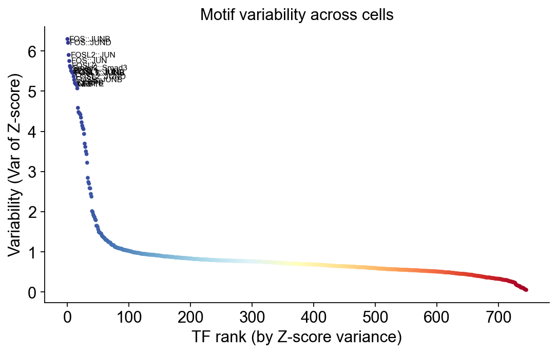
TF variability (ArchR plotVarDev) — a rank plot of motifs by variance of Z-score across cells. The top of this list is where you look for interesting TFs.
UMAP coloured by TF Z-score — the classic “is this TF active in cluster X?” sanity check.
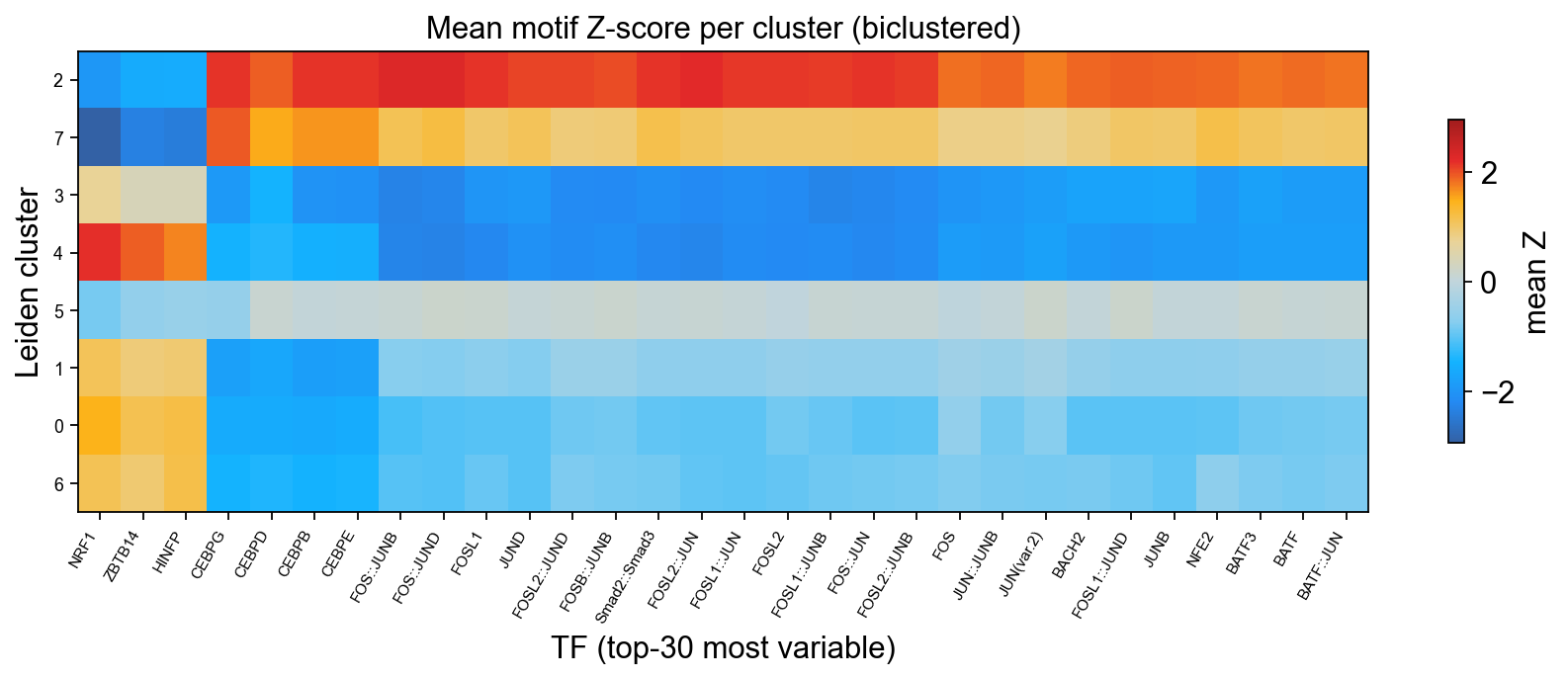
Cluster × TF heatmap — mean Z-score per (cluster, top-TF), biclustered so co-regulated TF modules and related clusters cluster together.

Variability is computed as the variance of each motif’s Z-scores across all cells: TFs whose activity is similar in every cell get a low score (uninformative), TFs whose activity separates populations get a high one.

# Load ArchR-style palettes from Epione.
from epione.pl._peak2gene import ARCHR_STALLION

ARCHR_SOLAR = mpl.colors.LinearSegmentedColormap.from_list(
    'archr_solar',
    ['#3361A5', '#248AF3', '#14B3FF', '#88CEEF', '#C1D5DC',
     '#EAD397', '#FDB31A', '#E42A2A', '#A31D1D'],
)

# Variance of Z-score across cells, then sort motifs by descending variance.
variability = np.nanvar(Z, axis=0)
rank = np.argsort(-variability)

# JASPAR motif IDs come through as e.g. "MA0492.1_JUND". Strip the ID prefix
# so the plots show just the TF name.
def tf_name(n):
    s = str(n)
    return s.split('_', 1)[-1] if '_' in s else s

print('Top 10 most-variable motifs:')
for r in rank[:10]:
    print(f'  {tf_name(names[r])}  (var={variability[r]:.2f})')

Top 10 most-variable motifs:
  FOS::JUNB  (var=6.30)
  FOS::JUND  (var=6.21)
  FOSL2::JUN  (var=5.90)
  FOS::JUN  (var=5.75)
  FOSL2  (var=5.63)
  Smad2::Smad3  (var=5.59)
  FOSL1  (var=5.51)
  FOSL1::JUN  (var=5.49)
  FOSL1::JUNB  (var=5.46)
  FOSL2::JUNB  (var=5.46)

Plot 1 · TF variability (`plotVarDev`)#

Each point is one motif, ranked by Z-score variance across cells. The top 15 are labelled. Lineage-defining TFs (e.g. EBF1, PAX5 for B cells, GATA3 for T, CEBPB for monocytes in PBMC) should sit at the top.

fig, ax = plt.subplots(figsize=(7, 4.5))

# x axis = rank, y axis = variance. Color by rank so the plot has a clean
# colour gradient from blue (high variance) → red (low variance).
x_rank = np.arange(len(variability))
y_var = variability[rank]
colors = plt.cm.RdYlBu_r(np.linspace(0, 1, len(x_rank)))
ax.scatter(x_rank, y_var, c=colors, s=6)

# Label the top 15.
for i in range(15):
    ax.text(x_rank[i] + 3, y_var[i], tf_name(names[rank[i]]),
            fontsize=7, va='center', ha='left')

ax.set_xlabel('TF rank (by Z-score variance)')
ax.set_ylabel('Variability (Var of Z-score)')
ax.set_title('Motif variability across cells')
ax.spines[['top', 'right']].set_visible(False)

plt.tight_layout()
display(fig)
plt.close(fig)

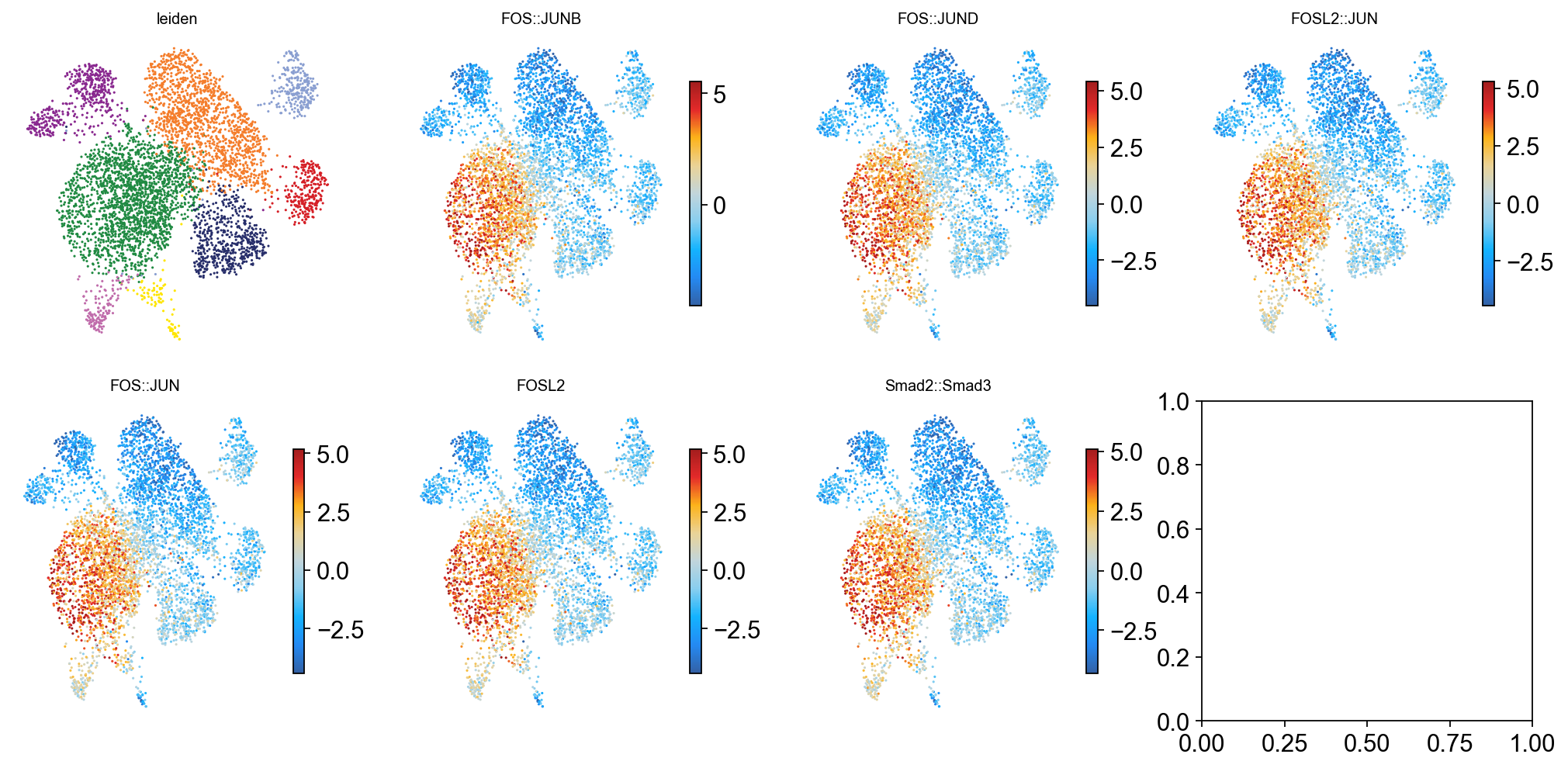
../../_images/ab33fa90d64d88cfa91b25281b67bfccbe6d009c72e618f46afee38ddb5fa539.png

Plot 2 · UMAP coloured by TF Z-score#

We show the Leiden clustering (panel 1) alongside the UMAP coloured by Z-score for each of the top-6 most-variable TFs (panels 2–7). Z-score is clipped to the 1–99 % range before colouring to keep outliers from washing out the palette.

# Grab UMAP coordinates + pick the top-k variable TFs.
top_k = 6
umap = adata.obsm['X_umap']
top_tfs = [names[rank[i]] for i in range(top_k)]

# Stash each top-k Z-score as a one-column .obs series — just used for
# the colouring below.
for tf in top_tfs:
    j = np.where(names == tf)[0][0]
    adata.obs[tf] = Z[:, j]

panels = ['leiden'] + top_tfs
ncols = (len(panels) + 1) // 2
fig, axes = plt.subplots(2, ncols, figsize=(3.2 * ncols, 6.4))
axes = axes.ravel()

for i, col in enumerate(panels):
    ax = axes[i]
    if col == 'leiden':
        # Categorical palette from ARCHR_STALLION.
        cats = adata.obs['leiden'].astype('category').cat.categories
        palette = {c: ARCHR_STALLION[k % len(ARCHR_STALLION)]
                   for k, c in enumerate(cats)}
        c_vals = adata.obs['leiden'].map(palette).values
        ax.scatter(umap[:, 0], umap[:, 1], c=c_vals, s=2, linewidths=0)
        ax.set_title('leiden', fontsize=9)
    else:
        vals = adata.obs[col].to_numpy(dtype=np.float32)
        lo, hi = np.nanpercentile(vals, [1, 99])
        sc_ = ax.scatter(
            umap[:, 0], umap[:, 1], c=vals, s=2, linewidths=0,
            cmap=ARCHR_SOLAR, vmin=lo, vmax=hi,
        )
        ax.set_title(tf_name(col), fontsize=9)
        plt.colorbar(sc_, ax=ax, shrink=0.7)
    ax.set_xticks([]); ax.set_yticks([])
    ax.spines[:].set_visible(False)

plt.tight_layout()
display(fig)
plt.close(fig)

../../_images/8a1067c991c99c0b2028ee51f972df1ab8a1be4b463122f2c2ace37cd376ab9f.png

Plot 3 · Cluster × TF heatmap (`plotMarkerHeatmap`)#

Mean Z-score per (Leiden cluster, top-30 variable TF), with both rows (clusters) and columns (TFs) biclustered via Ward linkage so that related clusters and co-activated TF modules appear next to each other. The diverging ARCHR_SOLAR colormap is centred at zero — blue = TF depleted, red = TF enriched.

import scipy.cluster.hierarchy as sch

# Mean Z-score per (cluster, TF) for the top-30 most-variable TFs.
top_n = 30
tf_idx = rank[:top_n]
group = adata.obs['leiden'].astype('category')
cats = list(group.cat.categories)

heat = np.stack([
    np.nanmean(Z[group.values == c][:, tf_idx], axis=0)
    for c in cats
])  # shape: (n_clusters, top_n)

# Ward-linkage bicluster.
link_rows = sch.linkage(heat.T, method='ward')
link_cols = sch.linkage(heat,   method='ward')
row_order = sch.leaves_list(link_rows)
col_order = sch.leaves_list(link_cols)

H = heat[col_order][:, row_order]
tf_labels = [tf_name(names[tf_idx[i]]) for i in row_order]
cluster_labels = [cats[i] for i in col_order]

# Plot.
fig, ax = plt.subplots(figsize=(11, 4.5))
vmax = float(np.nanmax(np.abs(H)))  # symmetric diverging range
im = ax.imshow(H, aspect='auto', cmap=ARCHR_SOLAR,
               vmin=-vmax, vmax=vmax, interpolation='nearest')

ax.set_yticks(range(len(cluster_labels)))
ax.set_yticklabels(cluster_labels, fontsize=8)
ax.set_xticks(range(len(tf_labels)))
ax.set_xticklabels(tf_labels, rotation=60, ha='right', fontsize=7)
ax.set_xlabel('TF (top-30 most variable)')
ax.set_ylabel('Leiden cluster')
ax.set_title('Mean motif Z-score per cluster (biclustered)')

plt.colorbar(im, ax=ax, shrink=0.7, label='mean Z')
plt.tight_layout()
display(fig)
plt.close(fig)

../../_images/e899e2c2f52cf89eedf87928042a5277bae6b63221bf566bfafaa891d89b64af.png

Notes and references#

The pre-built motif database scales across datasets: once you have motif_db_hg38_jaspar2020_5e5/ you can annotate any hg38 peak panel in under a second.
compute_deviations also stores the uncorrected deviation (obs_dev − mean(bg_dev), no standardisation) in adata.obsm['motif_deviations_raw']. Use that if you need the raw signal magnitude, not Z-scores.
If you need bit-level reproducibility with the original chromVAR or ArchR binaries, use method='sample'. On the ArchR heme benchmark the analytical vs. sample per-TF Pearson is ≥ 0.995 at ≥ 1 k cells — well within chromVAR’s own $1/\sqrt{n_{\mathrm{iter}}}$ sampling noise — but method='sample' matches ArchR’s numbers byte-for-byte when seeded identically.

References#

Schep AN, Wu B, Buenrostro JD, Greenleaf WJ. chromVAR: inferring transcription-factor-associated accessibility from single-cell epigenomic data. Nat Methods (2017).
Granja JM et al. ArchR is a scalable software package for integrative single-cell chromatin accessibility analysis. Nat Genet (2021).