Upstream tutorial: bulk ATAC-seq

Upstream tutorial: bulk ATAC-seq#

This notebook is an epione-native rewrite of the Galaxy Training Network ATAC-seq lesson. The biological aim is the same as in the GTN tutorial: start from paired-end ATAC FASTQs, align them to a reference genome, generate signal tracks, call peaks, and inspect whether the resulting data show the expected structure around a representative genomic locus and around transcription start sites.

What changes here is the execution model. Galaxy teaches the workflow as a sequence of web tools and dataset collections, whereas this notebook teaches the same logic through epi.upstream.* functions. The notebook is therefore meant to serve two roles at once:

Role	What it gives you
Executable tutorial	A small, public, end-to-end example that runs locally in the `omicdev` environment.
Project template	A direct prototype for replacing the toy FASTQs with real OTX2 samples while keeping the same `epione` API.

The underlying teaching dataset is the downsampled GTN ATAC example enriched for chr22. To keep the notebook genuinely runnable, we also build a lightweight chr22 demo reference from a locally cached GRCh38 FASTA. That makes the example much smaller than a full human run, but still preserves the same upstream concepts: alignment, filtering, fragment generation, Tn5 shifting, coverage export, peak calling, browser-style visualisation, and TSS-centred signal summarisation.

Scope note. This notebook covers the upstream part of a bulk ATAC-seq workflow: FASTQ -> filtered BAM -> fragments -> shifted BAM -> bigWig -> peaks -> visual QC. It does not cover downstream differential accessibility, motif analysis, or integration with RNA-seq.

Data provenance#

The example FASTQs are the public teaching files from the Galaxy Training Network ATAC-seq tutorial. In the GTN lesson they are used to demonstrate end-to-end preprocessing on a compact dataset that can be inspected interactively.

For this notebook we keep the same teaching logic but change the interface:

Item	Source	How it is used here
Paired-end FASTQs	Galaxy GTN ATAC tutorial toy dataset	Demonstrates the full upstream pipeline from alignment to peak calling.
GRCh38 FASTA	Local cache on this machine	Used to derive a small `chr22` reference so the notebook remains executable.
Galaxy locus	The `RAC2 / SSTR3` region shown in the GTN tutorial	Reused for locus-level visualization with `epi.bulk.bigwig`.

Local paths used throughout the notebook:

case/otx2/galaxy_atac_demo/
  fastq/     # downloaded GTN toy FASTQs
  ref/       # chr22 FASTA + bowtie2 index + derived annotation
  result/    # BAMs, fragments, bigWigs, MACS2 peaks

Learning goals#

By the end of the notebook, you should be able to answer five practical questions:

What is the minimal set of tools an epione ATAC-seq upstream run depends on?
How do epi.upstream.bowtie2.align_fastq_to_bam, epi.upstream.samtools.filter_bam, and epi.upstream.pipeline.bam_to_frags define the generic FASTQ -> BAM -> fragments backbone?
Why does ATAC-seq add an explicit epi.upstream.atac.shift_atac_bam step before coverage export?
How do we turn a processed ATAC BAM into interpretable peak and bigWig outputs?
How can the same explicit epione.upstream steps be transferred from a toy teaching example to real OTX2 samples?

import os
import pathlib
import urllib.request
import warnings

import pandas as pd
import epione as epi

warnings.filterwarnings('ignore', message='Function .* is missing a docstring.*')
os.environ['LC_ALL'] = 'C'
os.environ['LC_CTYPE'] = 'C'

epi.pl.plot_set()

WORK = pathlib.Path.cwd()
DATA = WORK / 'galaxy_atac_demo'
FASTQ_DIR = DATA / 'fastq'
REF_DIR = DATA / 'ref'
OUT = DATA / 'result'
for p in [FASTQ_DIR, REF_DIR, OUT]:
    p.mkdir(parents=True, exist_ok=True)

# Reuse the locally cached GRCh38 FASTA, but build a chr22-only demo reference
# so the tutorial remains lightweight enough to execute end-to-end.
HG38_FASTA = pathlib.Path('/scratch/users/steorra/data/snapatac2_cache/gencode_v41_GRCh38.fa.gz.decomp')
CHR22_FASTA = REF_DIR / 'chr22.fa'
CHR22_BT2_PREFIX = REF_DIR / 'chr22'
CHR22_SIZE = 50818468

ATAC_URLS = {
    'SRR891268_chr22_enriched_R1.fastq.gz': 'https://zenodo.org/record/3862793/files/SRR891268_chr22_enriched_R1.fastq.gz',
    'SRR891268_chr22_enriched_R2.fastq.gz': 'https://zenodo.org/record/3862793/files/SRR891268_chr22_enriched_R2.fastq.gz',
}

└─ 🔬 Starting plot initialization...
  ├─ Apply Scanpy/matplotlib settings
  ├─ Custom font setup
  ├─ Suppress warnings
  ├─ 
___________      .__                      
\_   _____/_____ |__| ____   ____   ____  
 |    __)_\____ \|  |/  _ \ /    \_/ __ \ 
 |        \  |_> >  (  <_> )   |  \  ___/ 
/_______  /   __/|__|\____/|___|  /\___  >
        \/|__|                  \/     \/ 

  ├─ 🔖 Version: 0.0.1rc1   📚 Tutorials: https://epione.readthedocs.io/
└─ ✅ plot_set complete.

1. Check upstream tools#

The Galaxy tutorial distributes preprocessing across several web tools, which makes it easy to forget that an ATAC-seq upstream workflow still depends on a fairly standard command-line stack under the hood. Before we touch the reads, we therefore make the dependency surface explicit.

For this notebook the critical components are:

Tool family	Why it matters
`bowtie2`	Aligns the paired-end ATAC reads to the reference genome.
`samtools`	Sorts, filters, and indexes BAM files.
`bedtools`	Supports fragment and interval-style conversions.
`MACS2`	Calls open chromatin peaks from the shifted ATAC alignments.
`epione` built-in implementations	Default Tn5 shifting and bigWig generation used directly inside the Python workflow.

epione wraps these tools, but it does not make their role disappear. Running a concise dependency check up front makes the notebook easier to debug and also mirrors good project hygiene: if the environment is inconsistent, it is better to learn that in seconds rather than after alignment has already run for several minutes.

epi.upstream.check_tools([
    'bowtie2',
    'samtools',
    'bedtools',
    'macs2',
])

✓  bowtie2                    /scratch/users/steorra/env/omicdev/bin/bowtie2
  ✓  samtools                   /scratch/users/steorra/env/omicdev/bin/samtools
  ✓  bedtools                   /scratch/users/steorra/env/omicdev/bin/bedtools
  ✓  macs2                      /scratch/users/steorra/env/omicdev/bin/macs2

{'bowtie2': '/scratch/users/steorra/env/omicdev/bin/bowtie2',
 'samtools': '/scratch/users/steorra/env/omicdev/bin/samtools',
 'bedtools': '/scratch/users/steorra/env/omicdev/bin/bedtools',
 'macs2': '/scratch/users/steorra/env/omicdev/bin/macs2'}

2. Download the Galaxy toy FASTQs#

The input files are the small paired-end FASTQs distributed with the Galaxy GTN ATAC-seq tutorial. They are downsampled and focused enough to support a complete teaching run while still containing the core structure of a real ATAC dataset.

Why use the Galaxy files instead of an arbitrary demo pair?

They are already tied to a published teaching narrative.
They are small enough to run repeatedly in a notebook.
They support a known locus-level example on chr22.
They make it easier to compare the epione output with the logic of the original GTN lesson.

At this stage we are only establishing the raw inputs. The important check is simply that the expected R1 and R2 files exist on disk and can now be passed to epi.upstream.* functions without any manual dataset bookkeeping.

for name, url in ATAC_URLS.items():
    out = FASTQ_DIR / name
    if not out.exists():
        print(f'downloading {name} ...')
        urllib.request.urlretrieve(url, out)
    else:
        print(f'skip existing: {name}')

fq1 = FASTQ_DIR / 'SRR891268_chr22_enriched_R1.fastq.gz'
fq2 = FASTQ_DIR / 'SRR891268_chr22_enriched_R2.fastq.gz'
pd.DataFrame({'fq1': [str(fq1)], 'fq2': [str(fq2)]})

downloading SRR891268_chr22_enriched_R1.fastq.gz ...
downloading SRR891268_chr22_enriched_R2.fastq.gz ...

	fq1	fq2
0	/scratch/users/steorra/analysis/omicverse_dev/...	/scratch/users/steorra/analysis/omicverse_dev/...

3. Prepare a `chr22` demo reference#

The original Galaxy tutorial is framed as a human-genome ATAC workflow, but the teaching plots focus on a chromosome 22 locus. For a notebook that must be executable from start to finish, building a full human bowtie2 index would be unnecessary overhead. We therefore construct a compact teaching reference containing only chr22.

This is a deliberate distinction between tutorial engineering and biological best practice:

Scenario	Recommended reference
Notebook demo / teaching run	A reduced `chr22` reference to keep runtime and disk use small.
Real project analysis	A full genome index matching the species, assembly, and annotation used in the study.

The epi.upstream.prepare_reference call encapsulates the reference-preparation step that is often scattered across shell scripts. Its main job is to ensure that the FASTA, chromosome sizes, and aligner index are all present in a form the later upstream functions can consume directly.

%%time
from pyfaidx import Fasta

if not CHR22_FASTA.exists():
    fa = Fasta(str(HG38_FASTA))
    with open(CHR22_FASTA, 'w') as fout:
        fout.write('>chr22\n')
        seq = str(fa['chr22'])
        for i in range(0, len(seq), 60):
            fout.write(seq[i:i+60] + '\n')

ref = epi.upstream.prepare_reference(
    fasta=CHR22_FASTA,
    aligner='bowtie2',
    index_prefix=CHR22_BT2_PREFIX,
)
ref

Settings:
  Output files: "/scratch/users/steorra/analysis/omicverse_dev/epione/epione_guide/tutorials/bulk/galaxy_atac_demo/ref/chr22.*.bt2"
  Line rate: 6 (line is 64 bytes)
  Lines per side: 1 (side is 64 bytes)
  Offset rate: 4 (one in 16)
  FTable chars: 10
  Strings: unpacked
  Max bucket size: default
  Max bucket size, sqrt multiplier: default
  Max bucket size, len divisor: 4
  Difference-cover sample period: 1024
  Endianness: little
  Actual local endianness: little
  Sanity checking: disabled
  Assertions: disabled
  Random seed: 0
  Sizeofs: void*:8, int:4, long:8, size_t:8
Input files DNA, FASTA:
  /scratch/users/steorra/analysis/omicverse_dev/epione/epione_guide/tutorials/bulk/galaxy_atac_demo/ref/chr22.fa
Reading reference sizes
Time reading reference sizes: 00:00:00
Calculating joined length
Writing header
Reserving space for joined string
Joining reference sequences
  Time to join reference sequences: 00:00:00
bmax according to bmaxDivN setting: 9789944
Using parameters --bmax 7342458 --dcv 1024
  Doing ahead-of-time memory usage test
  Passed!  Constructing with these parameters: --bmax 7342458 --dcv 1024
Constructing suffix-array element generator
Building DifferenceCoverSample
  Building sPrime
  Building sPrimeOrder
  V-Sorting samples
V-Sorting samples time: 00:00:00
  Allocating rank array
  Ranking v-sort output
  Ranking v-sort output time: 00:00:01
  Invoking Larsson-Sadakane on ranks
Invoking Larsson-Sadakane on ranks time: 00:00:00
  Sanity-checking and returning
Building samples
Reserving space for 12 sample suffixes
Generating random suffixes
QSorting 12 sample offsets, eliminating duplicates
QSorting sample offsets, eliminating duplicates time: 00:00:00
Multikey QSorting 12 samples
  (Using difference cover)
  Multikey QSorting samples time: 00:00:00
Calculating bucket sizes
Splitting and merging
  Splitting and merging time: 00:00:00
Avg bucket size: 4.89497e+06 (target: 7342457)
Converting suffix-array elements to index image
Allocating ftab, absorbFtab
Entering Ebwt loop
Getting block 1 of 8
  Reserving size (7342458) for bucket 1
  Calculating Z arrays for bucket 1
  Entering block accumulator loop for bucket 1:
  bucket 1: 10%
  bucket 1: 20%
  bucket 1: 30%
  bucket 1: 40%
  bucket 1: 50%
bucket 1: 60%
  bucket 1: 70%
  bucket 1: 80%
  bucket 1: 90%
  bucket 1: 100%
  Sorting block of length 6109124 for bucket 1
  (Using difference cover)
Sorting block time: 00:00:01
Returning block of 6109125 for bucket 1
Getting block 2 of 8
  Reserving size (7342458) for bucket 2
  Calculating Z arrays for bucket 2
  Entering block accumulator loop for bucket 2:
  bucket 2: 10%
  bucket 2: 20%
  bucket 2: 30%
  bucket 2: 40%
bucket 2: 50%
  bucket 2: 60%
  bucket 2: 70%
  bucket 2: 80%
  bucket 2: 90%
bucket 2: 100%
  Sorting block of length 4162165 for bucket 2
  (Using difference cover)
Sorting block time: 00:00:01
Returning block of 4162166 for bucket 2
Getting block 3 of 8
  Reserving size (7342458) for bucket 3
  Calculating Z arrays for bucket 3
  Entering block accumulator loop for bucket 3:
  bucket 3: 10%
bucket 3: 20%
  bucket 3: 30%
  bucket 3: 40%
  bucket 3: 50%
  bucket 3: 60%
bucket 3: 70%
  bucket 3: 80%
  bucket 3: 90%
  bucket 3: 100%
  Sorting block of length 3242487 for bucket 3
  (Using difference cover)
Sorting block time: 00:00:00
Returning block of 3242488 for bucket 3
Getting block 4 of 8
  Reserving size (7342458) for bucket 4
  Calculating Z arrays for bucket 4
  Entering block accumulator loop for bucket 4:
  bucket 4: 10%
bucket 4: 20%
  bucket 4: 30%
  bucket 4: 40%
  bucket 4: 50%
bucket 4: 60%
  bucket 4: 70%
  bucket 4: 80%
  bucket 4: 90%
bucket 4: 100%
  Sorting block of length 5059508 for bucket 4
  (Using difference cover)
Sorting block time: 00:00:00
Returning block of 5059509 for bucket 4
Getting block 5 of 8
  Reserving size (7342458) for bucket 5
  Calculating Z arrays for bucket 5
  Entering block accumulator loop for bucket 5:
bucket 5: 10%
  bucket 5: 20%
  bucket 5: 30%
  bucket 5: 40%
bucket 5: 50%
  bucket 5: 60%
  bucket 5: 70%
  bucket 5: 80%
bucket 5: 90%
  bucket 5: 100%
  Sorting block of length 2717729 for bucket 5
  (Using difference cover)
Sorting block time: 00:00:00
Returning block of 2717730 for bucket 5
Getting block 6 of 8
  Reserving size (7342458) for bucket 6
  Calculating Z arrays for bucket 6
  Entering block accumulator loop for bucket 6:
  bucket 6: 10%
  bucket 6: 20%
bucket 6: 30%
  bucket 6: 40%
  bucket 6: 50%
  bucket 6: 60%
bucket 6: 70%
  bucket 6: 80%
  bucket 6: 90%
  bucket 6: 100%
  Sorting block of length 6052533 for bucket 6
  (Using difference cover)
Sorting block time: 00:00:01
Returning block of 6052534 for bucket 6
Getting block 7 of 8
  Reserving size (7342458) for bucket 7
  Calculating Z arrays for bucket 7
  Entering block accumulator loop for bucket 7:
  bucket 7: 10%
  bucket 7: 20%
  bucket 7: 30%
bucket 7: 40%
  bucket 7: 50%
  bucket 7: 60%
  bucket 7: 70%
bucket 7: 80%
  bucket 7: 90%
  bucket 7: 100%
  Sorting block of length 6696876 for bucket 7
  (Using difference cover)
Sorting block time: 00:00:01
Returning block of 6696877 for bucket 7
Getting block 8 of 8
  Reserving size (7342458) for bucket 8
  Calculating Z arrays for bucket 8
  Entering block accumulator loop for bucket 8:
  bucket 8: 10%
  bucket 8: 20%
  bucket 8: 30%
  bucket 8: 40%
  bucket 8: 50%
  bucket 8: 60%
bucket 8: 70%
  bucket 8: 80%
  bucket 8: 90%
  bucket 8: 100%
  Sorting block of length 5119348 for bucket 8
  (Using difference cover)
Sorting block time: 00:00:01
Returning block of 5119349 for bucket 8
Exited Ebwt loop
fchr[A]: 0
fchr[C]: 10382214
fchr[G]: 19542866
fchr[T]: 28789052
fchr[$]: 39159777
Exiting Ebwt::buildToDisk()
Returning from initFromVector
Wrote 17248347 bytes to primary EBWT file: /scratch/users/steorra/analysis/omicverse_dev/epione/epione_guide/tutorials/bulk/galaxy_atac_demo/ref/chr22.1.bt2.tmp
Wrote 9789952 bytes to secondary EBWT file: /scratch/users/steorra/analysis/omicverse_dev/epione/epione_guide/tutorials/bulk/galaxy_atac_demo/ref/chr22.2.bt2.tmp
Re-opening _in1 and _in2 as input streams
Returning from Ebwt constructor
Headers:
    len: 39159777
    bwtLen: 39159778
    sz: 9789945
    bwtSz: 9789945
    lineRate: 6
    offRate: 4
    offMask: 0xfffffff0
    ftabChars: 10
    eftabLen: 20
    eftabSz: 80
    ftabLen: 1048577
    ftabSz: 4194308
    offsLen: 2447487
    offsSz: 9789948
    lineSz: 64
    sideSz: 64
    sideBwtSz: 48
    sideBwtLen: 192
    numSides: 203958
    numLines: 203958
    ebwtTotLen: 13053312
    ebwtTotSz: 13053312
    color: 0
    reverse: 0
Total time for call to driver() for forward index: 00:00:12
Reading reference sizes
Time reading reference sizes: 00:00:00
Calculating joined length
Writing header
Reserving space for joined string
Joining reference sequences
  Time to join reference sequences: 00:00:00
  Time to reverse reference sequence: 00:00:00
bmax according to bmaxDivN setting: 9789944
Using parameters --bmax 7342458 --dcv 1024
  Doing ahead-of-time memory usage test
  Passed!  Constructing with these parameters: --bmax 7342458 --dcv 1024
Constructing suffix-array element generator
Building DifferenceCoverSample
  Building sPrime
  Building sPrimeOrder
  V-Sorting samples
V-Sorting samples time: 00:00:01
  Allocating rank array
  Ranking v-sort output
  Ranking v-sort output time: 00:00:00
  Invoking Larsson-Sadakane on ranks
Invoking Larsson-Sadakane on ranks time: 00:00:00
  Sanity-checking and returning
Building samples
Reserving space for 12 sample suffixes
Generating random suffixes
QSorting 12 sample offsets, eliminating duplicates
QSorting sample offsets, eliminating duplicates time: 00:00:00
Multikey QSorting 12 samples
  (Using difference cover)
  Multikey QSorting samples time: 00:00:00
Calculating bucket sizes
Splitting and merging
  Splitting and merging time: 00:00:00
Avg bucket size: 5.59425e+06 (target: 7342457)
Converting suffix-array elements to index image
Allocating ftab, absorbFtab
Entering Ebwt loop
Getting block 1 of 7
  Reserving size (7342458) for bucket 1
  Calculating Z arrays for bucket 1
  Entering block accumulator loop for bucket 1:
  bucket 1: 10%
  bucket 1: 20%
  bucket 1: 30%
  bucket 1: 40%
  bucket 1: 50%
  bucket 1: 60%
bucket 1: 70%
  bucket 1: 80%
  bucket 1: 90%
  bucket 1: 100%
  Sorting block of length 6882572 for bucket 1
  (Using difference cover)
Sorting block time: 00:00:01
Returning block of 6882573 for bucket 1
Getting block 2 of 7
  Reserving size (7342458) for bucket 2
  Calculating Z arrays for bucket 2
  Entering block accumulator loop for bucket 2:
  bucket 2: 10%
  bucket 2: 20%
  bucket 2: 30%
  bucket 2: 40%
bucket 2: 50%
  bucket 2: 60%
  bucket 2: 70%
  bucket 2: 80%
  bucket 2: 90%
bucket 2: 100%
  Sorting block of length 7217801 for bucket 2
  (Using difference cover)
Sorting block time: 00:00:01
Returning block of 7217802 for bucket 2
Getting block 3 of 7
  Reserving size (7342458) for bucket 3
  Calculating Z arrays for bucket 3
  Entering block accumulator loop for bucket 3:
  bucket 3: 10%
  bucket 3: 20%
  bucket 3: 30%
bucket 3: 40%
  bucket 3: 50%
  bucket 3: 60%
  bucket 3: 70%
bucket 3: 80%
  bucket 3: 90%
  bucket 3: 100%
  Sorting block of length 6398765 for bucket 3
  (Using difference cover)
Sorting block time: 00:00:01
Returning block of 6398766 for bucket 3
Getting block 4 of 7
  Reserving size (7342458) for bucket 4
  Calculating Z arrays for bucket 4
  Entering block accumulator loop for bucket 4:
  bucket 4: 10%
  bucket 4: 20%
bucket 4: 30%
  bucket 4: 40%
  bucket 4: 50%
  bucket 4: 60%
bucket 4: 70%
  bucket 4: 80%
  bucket 4: 90%
  bucket 4: 100%
  Sorting block of length 2716193 for bucket 4
  (Using difference cover)
Sorting block time: 00:00:01
Returning block of 2716194 for bucket 4
Getting block 5 of 7
  Reserving size (7342458) for bucket 5
  Calculating Z arrays for bucket 5
  Entering block accumulator loop for bucket 5:
  bucket 5: 10%
  bucket 5: 20%
bucket 5: 30%
  bucket 5: 40%
  bucket 5: 50%
  bucket 5: 60%
bucket 5: 70%
  bucket 5: 80%
  bucket 5: 90%
  bucket 5: 100%
  Sorting block of length 5106643 for bucket 5
  (Using difference cover)
Sorting block time: 00:00:01
Returning block of 5106644 for bucket 5
Getting block 6 of 7
  Reserving size (7342458) for bucket 6
  Calculating Z arrays for bucket 6
  Entering block accumulator loop for bucket 6:
bucket 6: 10%
  bucket 6: 20%
  bucket 6: 30%
  bucket 6: 40%
bucket 6: 50%
  bucket 6: 60%
  bucket 6: 70%
  bucket 6: 80%
bucket 6: 90%
  bucket 6: 100%
  Sorting block of length 6895232 for bucket 6
  (Using difference cover)
Sorting block time: 00:00:01
Returning block of 6895233 for bucket 6
Getting block 7 of 7
  Reserving size (7342458) for bucket 7
  Calculating Z arrays for bucket 7
  Entering block accumulator loop for bucket 7:
  bucket 7: 10%
  bucket 7: 20%
  bucket 7: 30%
  bucket 7: 40%
  bucket 7: 50%
  bucket 7: 60%
bucket 7: 70%
  bucket 7: 80%
  bucket 7: 90%
  bucket 7: 100%
  Sorting block of length 3942565 for bucket 7
  (Using difference cover)
Sorting block time: 00:00:01
Returning block of 3942566 for bucket 7
Exited Ebwt loop
fchr[A]: 0
fchr[C]: 10382214
fchr[G]: 19542866
fchr[T]: 28789052
fchr[$]: 39159777
Exiting Ebwt::buildToDisk()
Returning from initFromVector
Wrote 17248347 bytes to primary EBWT file: /scratch/users/steorra/analysis/omicverse_dev/epione/epione_guide/tutorials/bulk/galaxy_atac_demo/ref/chr22.rev.1.bt2.tmp
Wrote 9789952 bytes to secondary EBWT file: /scratch/users/steorra/analysis/omicverse_dev/epione/epione_guide/tutorials/bulk/galaxy_atac_demo/ref/chr22.rev.2.bt2.tmp
Re-opening _in1 and _in2 as input streams
Returning from Ebwt constructor
Headers:
    len: 39159777
    bwtLen: 39159778
    sz: 9789945
    bwtSz: 9789945
    lineRate: 6
    offRate: 4
    offMask: 0xfffffff0
    ftabChars: 10
    eftabLen: 20
    eftabSz: 80
    ftabLen: 1048577
    ftabSz: 4194308
    offsLen: 2447487
    offsSz: 9789948
    lineSz: 64
    sideSz: 64
    sideBwtSz: 48
    sideBwtLen: 192
    numSides: 203958
    numLines: 203958
    ebwtTotLen: 13053312
    ebwtTotSz: 13053312
    color: 0
    reverse: 1
Total time for backward call to driver() for mirror index: 00:00:12
CPU times: user 203 ms, sys: 95.5 ms, total: 299 ms
Wall time: 25.1 s

{'fasta': '/scratch/users/steorra/analysis/omicverse_dev/epione/epione_guide/tutorials/bulk/galaxy_atac_demo/ref/chr22.fa',
 'fai': '/scratch/users/steorra/analysis/omicverse_dev/epione/epione_guide/tutorials/bulk/galaxy_atac_demo/ref/chr22.fa.fai',
 'chrom_sizes': '/scratch/users/steorra/analysis/omicverse_dev/epione/epione_guide/tutorials/bulk/galaxy_atac_demo/ref/chr22.chrom.sizes',
 'ref_index': '/scratch/users/steorra/analysis/omicverse_dev/epione/epione_guide/tutorials/bulk/galaxy_atac_demo/ref/chr22'}

4. Build the generic paired-end backbone explicitly#

Instead of calling a single convenience wrapper, this notebook now spells out the reusable upstream backbone as separate epione.upstream operations. That makes the control points obvious:

epi.upstream.bowtie2.align_fastq_to_bam(...) performs the raw paired-end alignment and duplicate marking.
epi.upstream.samtools.filter_bam(...) applies the mapping-quality and flag filters that define the retained alignment set.
epi.upstream.samtools.index_bam(...) creates the BAM index needed for downstream random access.
epi.upstream.pipeline.bam_to_frags(...) converts the filtered paired-end BAM into a fragment table.

This decomposition is closer to how the workflow is reasoned about biologically. The fragment file is no longer a side effect of a wrapper. It is an explicit output produced from an explicit filtered BAM.

Why keep the fragment file?#

Even though the rest of the tutorial emphasizes signal tracks and peak calling, the fragment table remains valuable because it captures the retained paired-end molecules directly and can be reused in later accessibility analyses.

%%time
sample_name = 'SRR891268_galaxy_atac'
frag_dir = OUT / 'fragments'
frag_dir.mkdir(parents=True, exist_ok=True)
raw_bam = frag_dir / f'{sample_name}.raw.bam'
filt_bam = frag_dir / f'{sample_name}.filtered.bam'
frags_path = frag_dir / f'{sample_name}.frags.tsv.gz'

for stale in [raw_bam, filt_bam, pathlib.Path(str(filt_bam) + '.bai'), frags_path]:
    if stale.exists():
        stale.unlink()

epi.upstream.bowtie2.align_fastq_to_bam(
    fq1=str(fq1),
    fq2=str(fq2),
    out_bam=raw_bam,
    ref_index=ref['ref_index'],
    threads=8,
    extra_args=['--very-sensitive', '-X', '2000'],
    remove_duplicates=True,
)
epi.upstream.samtools.filter_bam(
    raw_bam,
    filt_bam,
    mapq=30,
    proper_pair=True,
    drop_secondary_supp=True,
    drop_duplicates=False,
    drop_qcfail=True,
    drop_unmapped=True,
    drop_mate_unmapped=True,
    drop_chroms=('chrM',),
    threads=8,
)
epi.upstream.samtools.index_bam(filt_bam, threads=8)
epi.upstream.pipeline.bam_to_frags(filt_bam, sample_name, frags_path)
raw_bam.unlink(missing_ok=True)

bam_path = str(filt_bam)
frags_path = str(frags_path)
{'bam': bam_path, 'frags': frags_path}

CPU times: user 2.97 ms, sys: 35.4 ms, total: 38.3 ms
Wall time: 16.1 s

{'bam': '/scratch/users/steorra/analysis/omicverse_dev/epione/epione_guide/tutorials/bulk/galaxy_atac_demo/result/fragments/SRR891268_galaxy_atac.filtered.bam',
 'frags': '/scratch/users/steorra/analysis/omicverse_dev/epione/epione_guide/tutorials/bulk/galaxy_atac_demo/result/fragments/SRR891268_galaxy_atac.frags.tsv.gz'}

5. Add the ATAC-specific processing steps explicitly#

The generic backbone above gives us a filtered paired-end BAM and a fragment table. ATAC-seq then adds one assay-specific transformation before browser-style visualization: Tn5 shifting.

Here the assay logic is again written as separate steps rather than hidden inside a high-level helper:

Operation	`epione` function	Why it matters
Tn5 offset correction	`epi.upstream.atac.shift_atac_bam(...)`	Moves aligned ends closer to the transposition event.
Coverage export	`epi.upstream.bigwig.bam_to_bigwig(...)`	Converts the shifted BAM into a signal track for plotting and matrix aggregation.

This layout makes the ATAC-specific part of the pipeline very clear: ATAC is just the generic paired-end backbone plus the shift step plus coverage export.

%%time
atac_dir = OUT / 'atac'
atac_dir.mkdir(parents=True, exist_ok=True)
shift_bam = atac_dir / f'{sample_name}.shift.bam'
atac_bw = atac_dir / f'{sample_name}.bw'
source_bam = OUT / 'fragments' / f'{sample_name}.filtered.bam'

for stale in [shift_bam, pathlib.Path(str(shift_bam) + '.bai'), atac_bw]:
    if stale.exists():
        stale.unlink()

epi.upstream.atac.shift_atac_bam(
    source_bam,
    shift_bam,
    threads=8,
    index=True,
)
epi.upstream.bigwig.bam_to_bigwig(
    shift_bam,
    atac_bw,
    bin_size=10,
    threads=8,
)

{
    'shift_bam': str(shift_bam),
    'bigwig': str(atac_bw),
}

CPU times: user 26.4 s, sys: 625 ms, total: 27.1 s
Wall time: 26.4 s

{'shift_bam': '/scratch/users/steorra/analysis/omicverse_dev/epione/epione_guide/tutorials/bulk/galaxy_atac_demo/result/atac/SRR891268_galaxy_atac.shift.bam',
 'bigwig': '/scratch/users/steorra/analysis/omicverse_dev/epione/epione_guide/tutorials/bulk/galaxy_atac_demo/result/atac/SRR891268_galaxy_atac.bw'}

6. Peak calling#

Once the shifted ATAC BAM is available, the next goal is to identify candidate accessible regions. In practical terms, this means converting the processed alignment into a standard peak set that can later be visualized, annotated, intersected with motifs, or compared across samples.

Why peak calling is still a separate step#

Coverage tracks are useful for visual interpretation, but they are not an analysis-ready set of regions. Peak calling imposes a statistical threshold and converts a continuous signal profile into a discrete list of candidate regulatory intervals.

The function#

epi.upstream.macs2.call_peaks_macs2(...) is the epione wrapper around MACS2 peak calling.

Key parameter	What it controls
`bam`	Input alignment used as the signal source.
`format='BAMPE'`	Treats the data as paired-end fragments rather than single-end reads.
`qvalue`	Reporting threshold for significant peaks.
`nomodel=True`	Skips model building, which is common for ATAC-seq workflows.

Because the executable notebook runs on a reduced chr22 reference, the goal is not to estimate a publication-ready regulatory catalogue. The goal is to produce a coherent toy peak set that can be interrogated visually.

%%time
sample_name = 'SRR891268_galaxy_atac'
shift_bam = OUT / 'atac' / f'{sample_name}.shift.bam'
if not shift_bam.exists():
    epi.upstream.atac.shift_atac_bam(
        OUT / 'fragments' / f'{sample_name}.filtered.bam',
        shift_bam,
        threads=8,
        index=True,
    )
peak_paths = epi.upstream.macs2.call_peaks_macs2(
    bam=shift_bam,
    out_dir=OUT / 'peaks',
    name=sample_name,
    genome_size='hs',
    format='BAMPE',
    qvalue=0.01,
    keep_dup='all',
    call_summits=True,
    nomodel=True,
)
peak_paths

CPU times: user 1.79 ms, sys: 1.04 ms, total: 2.83 ms
Wall time: 484 ms

{'narrowPeak': '/scratch/users/steorra/analysis/omicverse_dev/epione/epione_guide/tutorials/bulk/galaxy_atac_demo/result/peaks/SRR891268_galaxy_atac_peaks.narrowPeak',
 'summits': '/scratch/users/steorra/analysis/omicverse_dev/epione/epione_guide/tutorials/bulk/galaxy_atac_demo/result/peaks/SRR891268_galaxy_atac_summits.bed',
 'xls': '/scratch/users/steorra/analysis/omicverse_dev/epione/epione_guide/tutorials/bulk/galaxy_atac_demo/result/peaks/SRR891268_galaxy_atac_peaks.xls'}

Reading the peak output#

After MACS2 finishes, the result directory contains several standard files. The exact filenames are not the main lesson; the important point is what they mean:

File type	Interpretation
`*_peaks.narrowPeak`	Main interval set used for plotting and downstream analysis.
`*_summits.bed`	Local maxima within broader peak intervals.
`*_peaks.xls`	Verbose MACS2 report with scores and supporting statistics.

In a full project run you would now typically inspect peak counts, overlap with promoters or distal elements, and reproducibility across replicates. In this compact tutorial we instead carry the resulting peak intervals forward into a locus-level visualization step.

7. Visualise the Galaxy locus with `epi.bulk.bigwig`#

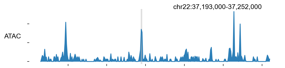
One of the strengths of the Galaxy ATAC tutorial is that it does not stop at file generation. It also shows how to read the output by looking at an instructive genomic locus. We keep exactly that teaching move here and reuse the same chr22:37,193,000-37,252,000 region near RAC2 / SSTR3.

Biological question#

Does the processed ATAC signal produce a coherent accessibility profile at this locus, and do the called peaks align with the strongest local enrichments in the bigWig track?

The function#

epi.bulk.bigwig(...).plot_track(...) renders browser-style signal tracks directly from bigWig files.

Key parameter	What it controls
`chrom`, `chromstart`, `chromend`	Genomic window shown in the plot.
`plot_names`	Which registered bigWig tracks to display.
`bp_per_bin`	Horizontal aggregation scale in base pairs.
`region_dict`	Highlight boxes marking intervals of special interest, here the MACS2 peaks.
`color_dict`	Per-track visual color mapping.

How to read the plot#

A useful browser panel should show agreement between the two representations of the data:

the continuous signal profile in the bigWig track, and
the discrete intervals in the peak set.

If the strongest called peaks sit on top of the strongest local coverage enrichments, the preprocessing chain has produced an internally consistent result.

ATAC_GALAXY_LOCUS = ('chr22', 37193000, 37252000)
atac_bigwig = str(OUT / 'atac' / 'SRR891268_galaxy_atac.bw')

bw_obj = epi.bulk.bigwig({'ATAC': atac_bigwig})
bw_obj.read()

peak_df = pd.read_csv(peak_paths['narrowPeak'], sep='	', header=None)
peak_df = peak_df[peak_df[0] == 'chr22'].copy()
peak_df = peak_df[(peak_df[1] < ATAC_GALAXY_LOCUS[2]) & (peak_df[2] > ATAC_GALAXY_LOCUS[1])]
region_dict = {
    f'peak_{i+1}': (int(r[1]), int(r[2]))
    for i, r in peak_df.head(8).iterrows()
}
color_dict = {'ATAC': '#2C7FB8'}

bw_obj.plot_track(
    chrom=ATAC_GALAXY_LOCUS[0],
    chromstart=ATAC_GALAXY_LOCUS[1],
    chromend=ATAC_GALAXY_LOCUS[2],
    plot_names=['ATAC'],
    figwidth=8,
    figheight=1.8,
    color_dict=color_dict,
    bp_per_bin=200,
    region_dict=region_dict,
)

└─ Load bigWig files
  └─ Loading ATAC...

(<Figure size 640x144 with 1 Axes>, [<Axes: ylabel='ATAC'>])

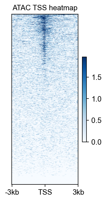
../../_images/82193795111a20254145940a7891d89ef46f1b575014c91196c64c27a956dc8d.png

8. Compute a TSS heatmap with `epi.bulk.bigwig`#

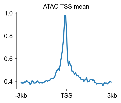
A locus snapshot is informative, but it is still a hand-picked view. To complement that local visualization, we also compute a TSS-centered heatmap and mean profile. This mirrors the signal-aggregation logic commonly taught in browser- or matrix-based genomics tutorials, but uses epione.bulk.bigwig directly.

Biological question#

Is accessibility enriched around transcription start sites in the processed ATAC bigWig, as we would expect for a plausible ATAC-seq dataset?

Why a temporary `chr22` annotation is created#

The notebook runs on a reduced chr22 reference, so we also derive a minimal transcript annotation from the local GRCh38 GENCODE gff3 file. That small GTF is not meant to replace a proper project annotation; it is only a lightweight teaching companion that lets the matrix computation stay consistent with the reduced demo reference.

The functions#

This section follows the same three-step logic as more elaborate epione visualization tutorials:

load_gtf(...) to register transcript coordinates.
compute_matrix(...) to aggregate signal around TSSs.
plot_matrix(...) and plot_matrix_line(...) to display the heatmap and the mean profile.

Output	What it tells you
TSS heatmap	Whether many genes show promoter-proximal enrichment rather than a flat background.
Mean profile	Whether the aggregate signal peaks around the TSS center.

Together with the browser panel above, this gives both a local and a global quality readout for the processed ATAC demo.

GENCODE_GFF3 = pathlib.Path('/scratch/users/steorra/data/snapatac2_cache/gencode_v41_GRCh38.gff3.gz')
CHR22_GTF = REF_DIR / 'gencode_v41_chr22.transcripts.gtf'

CHR22_GTF = pathlib.Path(
    epi.utils.convert_gff_to_gtf(
        GENCODE_GFF3,
        CHR22_GTF,
        feature_whitelist=['transcript'],
        seqname_whitelist=['chr22'],
    )
)

with open(CHR22_GTF) as fin:
    transcript_count = sum(1 for _ in fin)

print(CHR22_GTF, transcript_count)

└─ Converting GFF to GTF: /scratch/users/steorra/data/snapatac2_cache/gencode_v41_GRCh38.gff3.gz -> /scratch/users/steorra/analysis/omicverse_dev/epione/epione_guide/tutorials/bulk/galaxy_atac_demo/ref/gencode_v41_chr22.transcripts.gtf
└─ Wrote 3939 GTF records
/scratch/users/steorra/analysis/omicverse_dev/epione/epione_guide/tutorials/bulk/galaxy_atac_demo/ref/gencode_v41_chr22.transcripts.gtf 3939

atac_bigwig = str(OUT / 'atac' / 'SRR891268_galaxy_atac.bw')
atac_tss = epi.bulk.bigwig({'ATAC': atac_bigwig})
atac_tss.read()
atac_tss.load_gtf(str(CHR22_GTF))
atac_tss.compute_matrix('ATAC', nbins=100, upstream=3000, downstream=3000, n_jobs=1)

fig, ax = atac_tss.plot_matrix(
    bw_name='ATAC',
    bw_type='TSS',
    figsize=(2.4, 4.2),
    cmap='Blues',
    vmax='auto',
    vmin='auto',
    fontsize=11,
    title='ATAC TSS heatmap',
)

atac_tss.plot_matrix_line(
    bw_name='ATAC',
    bw_type='TSS',
    figsize=(3.2, 2.6),
    color='#2C7FB8',
    fontsize=11,
    title='ATAC TSS mean',
)

└─ Load bigWig files
  └─ Loading ATAC...
└─ Load GTF file
  ├─ Reading GTF...
  └─ Reading GTF file from /scratch/users/steorra/analysis/omicverse_dev/epione/epione_guide/tutorials/bulk/galaxy_atac_demo/ref/gencode_v41_chr22.transcripts.gtf...
  └─ GTF file read successfully
  └─ GTF loaded
└─ Compute matrix: ATAC
  ├─ Prepare features
  ├─ Build matrices
└─ Finalize
  └─ ATAC matrix finished
  └─ ATAC tss matrix in bw_tss_scores_dict[ATAC]
  └─ ATAC tes matrix in bw_tes_scores_dict[ATAC]
  └─ ATAC body matrix in bw_body_scores_dict[ATAC]

(<Figure size 256x208 with 1 Axes>, <Axes: title={'center': 'ATAC TSS mean'}>)

../../_images/dad34426c967fcb700246df6673ef2acb9c51e7dc57cf984292c916296920e32.png

../../_images/24c2a0ed5c94ae838bc84cea806d44e356acdd935c4ced9fe326cc86ead838c3.png

9. OTX2 project template#

The final code cell is intentionally not another toy-data exercise. Instead, it is the handoff from tutorial mode to project mode. Replace the GTN FASTQ paths with the real OTX2 inputs, point ref_index to the full production reference, and keep the same explicit sequence of epi.upstream.bowtie2, epi.upstream.samtools, epi.upstream.atac, epi.upstream.bigwig, and epi.upstream.macs2 calls.

The important point is that there is no notebook-only wrapper hiding the workflow. The tutorial path and the project path now share the same step-by-step API surface.

# sample_name = 'h_OTX2_day2_ATAC'
# out_dir = WORK / 'otx2_upstream' / sample_name
# out_dir.mkdir(parents=True, exist_ok=True)
# raw_bam = out_dir / f'{sample_name}.raw.bam'
# filt_bam = out_dir / f'{sample_name}.filtered.bam'
# frags = out_dir / f'{sample_name}.frags.tsv.gz'
# shift_bam = out_dir / f'{sample_name}.shift.bam'
# bw_path = out_dir / f'{sample_name}.bw'
#
# epi.upstream.bowtie2.align_fastq_to_bam(
#     fq1='/path/to/h_OTX2_day2_ATAC_R1.fastq.gz',
#     fq2='/path/to/h_OTX2_day2_ATAC_R2.fastq.gz',
#     out_bam=raw_bam,
#     ref_index='/path/to/full/genome/index/prefix',
#     threads=8,
#     extra_args=['--very-sensitive', '-X', '2000'],
#     remove_duplicates=True,
# )
# epi.upstream.samtools.filter_bam(
#     raw_bam,
#     filt_bam,
#     mapq=30,
#     proper_pair=True,
#     drop_secondary_supp=True,
#     drop_qcfail=True,
#     drop_unmapped=True,
#     drop_mate_unmapped=True,
#     drop_chroms=('chrM',),
#     threads=8,
# )
# epi.upstream.samtools.index_bam(filt_bam, threads=8)
# epi.upstream.pipeline.bam_to_frags(filt_bam, sample_name, frags)
# epi.upstream.atac.shift_atac_bam(filt_bam, shift_bam, threads=8, index=True)
# epi.upstream.bigwig.bam_to_bigwig(shift_bam, bw_path, bin_size=10, threads=8)
# peak_paths = epi.upstream.macs2.call_peaks_macs2(
#     bam=shift_bam,
#     out_dir=WORK / 'otx2_upstream' / 'peaks',
#     name=sample_name,
#     genome_size='hs',
#     format='BAMPE',
#     qvalue=0.01,
#     keep_dup='all',
#     call_summits=True,
#     nomodel=True,
# )

Upstream tutorial: bulk ATAC-seq

Contents

Upstream tutorial: bulk ATAC-seq#

Data provenance#

Learning goals#

1. Check upstream tools#

2. Download the Galaxy toy FASTQs#

3. Prepare a chr22 demo reference#

4. Build the generic paired-end backbone explicitly#

Why keep the fragment file?#

5. Add the ATAC-specific processing steps explicitly#

6. Peak calling#

Why peak calling is still a separate step#

The function#

Reading the peak output#

7. Visualise the Galaxy locus with epi.bulk.bigwig#

Biological question#

The function#

How to read the plot#

8. Compute a TSS heatmap with epi.bulk.bigwig#

Biological question#

Why a temporary chr22 annotation is created#

The functions#

9. OTX2 project template#

3. Prepare a `chr22` demo reference#

7. Visualise the Galaxy locus with `epi.bulk.bigwig`#

8. Compute a TSS heatmap with `epi.bulk.bigwig`#

Why a temporary `chr22` annotation is created#