Integrate Multi Samples

import epione as epi
import anndataoom as oom
import scanpy as sc
import matplotlib.pyplot as plt

epi.pl.plot_set()

%load_ext autoreload
%autoreload 2

└─ 🔬 Starting plot initialization...
  ├─ Apply Scanpy/matplotlib settings
  ├─ Custom font setup
  ├─ Suppress warnings
  ├─ 
___________      .__                      
\_   _____/_____ |__| ____   ____   ____  
 |    __)_\____ \|  |/  _ \ /    \_/ __ \ 
 |        \  |_> >  (  <_> )   |  \  ___/ 
/_______  /   __/|__|\____/|___|  /\___  >
        \/|__|                  \/     \/ 

  ├─ 🔖 Version: 0.0.1rc1   📚 Tutorials: https://epione.readthedocs.io/
└─ ✅ plot_set complete.

Data Preparation

Import Data

For scATAC-seq data, we recommend starting your analysis from the fragment.tsv file. This is because the peak contents in the Cellranger-ATAC output matrix are inconsistent. Although Epione provides a peak merging function, it is still advisable to begin your analysis from the fragment level.

files=[
    ('scATAC_BMMC_R1','data/scATAC_BMMC_R1.fragments.tsv.gz'),
    ('scATAC_CD34_BMMC_R1','data/scATAC_CD34_BMMC_R1.fragments.tsv.gz'),
    ('scATAC_PBMC_R1','data/scATAC_PBMC_R1.fragments.tsv.gz')
]

%%time
import pathlib
pathlib.Path('result').mkdir(exist_ok=True)
out_files = ['result/' + name + '.h5ad' for name, _ in files]
if all(pathlib.Path(f).exists() for f in out_files):
    adatas = [epi.utils.load(f) for f in out_files]
else:
    adatas = epi.pp.import_fragments(
        [fl for _, fl in files], file=out_files,
        chrom_sizes=epi.utils.genome.hg19,
        min_num_fragments=1000, sorted_by_barcode=False,
    )
adatas

└─ scanning data/scATAC_BMMC_R1.fragments.tsv.gz
└─ imported 5,000 cells  (16,560,340 unique fragments)
└─ scanning data/scATAC_CD34_BMMC_R1.fragments.tsv.gz
└─ imported 3,393 cells  (13,150,375 unique fragments)
└─ scanning data/scATAC_PBMC_R1.fragments.tsv.gz
└─ imported 2,496 cells  (11,501,080 unique fragments)
CPU times: user 46.8 s, sys: 365 ms, total: 47.2 s
Wall time: 48 s

[╭────────────────────────────────────────────────────────────────────────╮
 │ AnnDataOOM                               Rust · out-of-memory · backed │
 ├────────────────────────────────────────────────────────────────────────┤
 │                                                                        │
 │    5,000   ×   0                                                       │
 │    obs          vars                                                   │
 │                                                                        │
 │    csr_matrix · float32 · 0.0% density · ~0.0 MB/chunk (1,000 rows) ·  │
 │    scATAC_BMMC_R1.h5ad                                                 │
 │                                                                        │
 ├────────────────────────────────────────────────────────────────────────┤
 │ ▸ obs    (3)    n_fragment · frac_dup · frac_mito                      │
 │ ▸ var    (–)                                                           │
 │ ▸ obsm   (–)                                                           │
 │ ▸ varm   (–)                                                           │
 │ ▸ obsp   (–)                                                           │
 │ ▸ varp   (–)                                                           │
 │ ▸ layers (–)                                                           │
 │ ▸ raw    (–)                                                           │
 ╰────────────────────────────────────────────────────────────────────────╯,
 ╭────────────────────────────────────────────────────────────────────────╮
 │ AnnDataOOM                               Rust · out-of-memory · backed │
 ├────────────────────────────────────────────────────────────────────────┤
 │                                                                        │
 │    3,393   ×   0                                                       │
 │    obs          vars                                                   │
 │                                                                        │
 │    csr_matrix · float32 · 0.0% density · ~0.0 MB/chunk (1,000 rows) ·  │
 │    scATAC_CD34_BMMC_R1.h5ad                                            │
 │                                                                        │
 ├────────────────────────────────────────────────────────────────────────┤
 │ ▸ obs    (3)    n_fragment · frac_dup · frac_mito                      │
 │ ▸ var    (–)                                                           │
 │ ▸ obsm   (–)                                                           │
 │ ▸ varm   (–)                                                           │
 │ ▸ obsp   (–)                                                           │
 │ ▸ varp   (–)                                                           │
 │ ▸ layers (–)                                                           │
 │ ▸ raw    (–)                                                           │
 ╰────────────────────────────────────────────────────────────────────────╯,
 ╭────────────────────────────────────────────────────────────────────────╮
 │ AnnDataOOM                               Rust · out-of-memory · backed │
 ├────────────────────────────────────────────────────────────────────────┤
 │                                                                        │
 │    2,496   ×   0                                                       │
 │    obs          vars                                                   │
 │                                                                        │
 │    csr_matrix · float32 · 0.0% density · ~0.0 MB/chunk (1,000 rows) ·  │
 │    scATAC_PBMC_R1.h5ad                                                 │
 │                                                                        │
 ├────────────────────────────────────────────────────────────────────────┤
 │ ▸ obs    (3)    n_fragment · frac_dup · frac_mito                      │
 │ ▸ var    (–)                                                           │
 │ ▸ obsm   (–)                                                           │
 │ ▸ varm   (–)                                                           │
 │ ▸ obsp   (–)                                                           │
 │ ▸ varp   (–)                                                           │
 │ ▸ layers (–)                                                           │
 │ ▸ raw    (–)                                                           │
 ╰────────────────────────────────────────────────────────────────────────╯]

Merge data

It is important to note that we should perform quality control on each adata dataset individually. However, since this section focuses on how to integrate and analyze data, the next step is data merging.

%%time
# Concatenate the 3 per-sample AnnData objects into a single AnnData
# with obs['sample'] and ``<sample>#<barcode>`` barcodes. Also writes
# a merged bgzipped + tabix-indexed fragments file (cached).
data = epi.pp.concat_samples(
    adatas=adatas,
    sample_names=[name for name, _ in files],
    fragment_files=[fl for _, fl in files],
    combined_fragments='data/pbmc_combined.fragments.tsv.gz',
    chrom_sizes=epi.utils.genome.hg19,
)
data

└─ concat_samples: 10,889 cells across 3 sample(s)
CPU times: user 4.49 ms, sys: 1.01 ms, total: 5.5 ms
Wall time: 6.34 ms

AnnData object with n_obs × n_vars = 10889 × 0
    obs: 'n_fragment', 'frac_dup', 'frac_mito', 'sample'
    uns: 'files', 'reference_sequences'

Peak Calling

If we have already annotated the data, we can obtain more meaningful peaks during peak calling. However, we can also perform peak calling before annotation. This means that at Epione, the optimal approach is to conduct peak calling twice: once now and once after annotation.

%%time
# Per-sample MACS3 (cached — delete to force re-run).
import pathlib
_cache = 'data/macs3_per_sample.pkl'
if pathlib.Path(_cache).exists():
    data.uns['macs3_pseudobulk'] = epi.utils.load(_cache)
else:
    epi.single.macs3(data, groupby='sample')
    epi.utils.save(dict(data.uns['macs3_pseudobulk']), _cache)

└─ loaded pickle ← data/macs3_per_sample.pkl
CPU times: user 28.2 ms, sys: 21.9 ms, total: 50.1 ms
Wall time: 59.7 ms

%%time
merged_peaks = epi.utils.merge_peaks(data.uns['macs3_pseudobulk'], epi.utils.hg19)
merged_peaks.head()

└─ merged 129,750 non-overlapping peaks
CPU times: user 44.5 s, sys: 99.2 ms, total: 44.6 s
Wall time: 46.6 s

	chrom	start	end	Peaks	group
0	chr1	565053	565553	chr1:565053-565553	scATAC_PBMC_R1
1	chr1	569133	569633	chr1:569133-569633	scATAC_PBMC_R1
2	chr1	713811	714311	chr1:713811-714311	scATAC_PBMC_R1
3	chr1	752395	752895	chr1:752395-752895	scATAC_BMMC_R1
4	chr1	762612	763112	chr1:762612-763112	scATAC_PBMC_R1

%%time
# Cell × peak matrix (cached).
import pathlib
_cache = 'data/pbmc_peak_calling.h5ad'
if pathlib.Path(_cache).exists():
    peak_mat = epi.utils.load(_cache)
else:
    peak_mat = epi.pp.make_peak_matrix(data, use_rep=merged_peaks['Peaks'])
    epi.utils.save(peak_mat, _cache)
peak_mat

└─ loaded AnnData ← data/pbmc_peak_calling.h5ad  (10889, 129750)
CPU times: user 106 ms, sys: 218 ms, total: 324 ms
Wall time: 388 ms

AnnData object with n_obs × n_vars = 10889 × 129750
    obs: 'n_fragment', 'frac_dup', 'frac_mito', 'sample', 'celltype'
    uns: 'files', 'reference_sequences'
    obsm: 'X_lsi', 'X_lsi_harmony', 'X_umap'
    obsp: 'connectivities', 'distances'

Since we are using anndata-rs to read data stored on the hard disk, we need to perform a close operation to ensure data integrity and security.

# data.close() not needed for anndataoom — backed writes are flushed.

# peak_mat already cached in cell above (make_peak_matrix auto-writes).

Batch correction

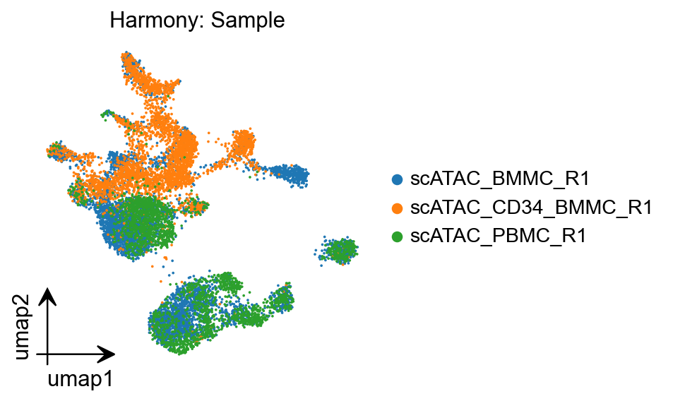
Sometimes the iterative LSI approach isnt enough of a correction for strong batch effect differences. For this reason, Epione implements a commonly used batch effect correction tool called Harmony which was originally designed for scRNA-seq. We provide a wrapper that will pass a dimensionality reduction object from Epione directly to the harmony function.

Harmony

epi.tl.lsi(
    peak_mat,
    n_components=100
)

└─ Starting optimized LSI analysis...
  └─ Computing TF-IDF normalization...
└─ Applying L1 normalization and log transformation...
└─ Performing randomized SVD...
└─ Standardizing embeddings...
  └─ Removing first component (typically associated with peak count per cell)
  └─ LSI analysis completed!

# Harmony integration of X_lsi across samples. scanpy 1.11+ +
# harmonypy 0.2 have a transposition mismatch (scanpy transposes
# harmonypy's Z_corr but Z_corr already ships as cells × features),
# so call harmonypy directly.
import harmonypy
_hm = harmonypy.run_harmony(
    peak_mat.obsm['X_lsi'].astype('float64'),
    peak_mat.obs, 'sample',
)
peak_mat.obsm['X_lsi_harmony'] = _hm.Z_corr
peak_mat

AnnData object with n_obs × n_vars = 10889 × 129750
    obs: 'n_fragment', 'frac_dup', 'frac_mito', 'sample', 'celltype'
    uns: 'files', 'reference_sequences'
    obsm: 'X_lsi', 'X_lsi_harmony', 'X_umap'
    obsp: 'connectivities', 'distances'

epi.pp.neighbors(peak_mat, use_rep="X_lsi_harmony", n_neighbors=15, n_pcs=30)
epi.tl.umap(peak_mat)

Computing neighbors with n_neighbors=15
Finished computing neighbors
    Added to .uns['neighbors']
    .obsp['distances'], distances for each pair of neighbors
    .obsp['connectivities'], weighted adjacency matrix
Computing UMAP embedding...
Finished computing UMAP
    Added:
        'X_umap', UMAP coordinates (adata.obsm)
        'umap', UMAP parameters (adata.uns)

%matplotlib inline
epi.pl.umap(
    peak_mat,
    #basis='X_umap',
    color='sample',
    title='Harmony: Sample',
    cmap='RdBu_r',
    vmin=0,
)

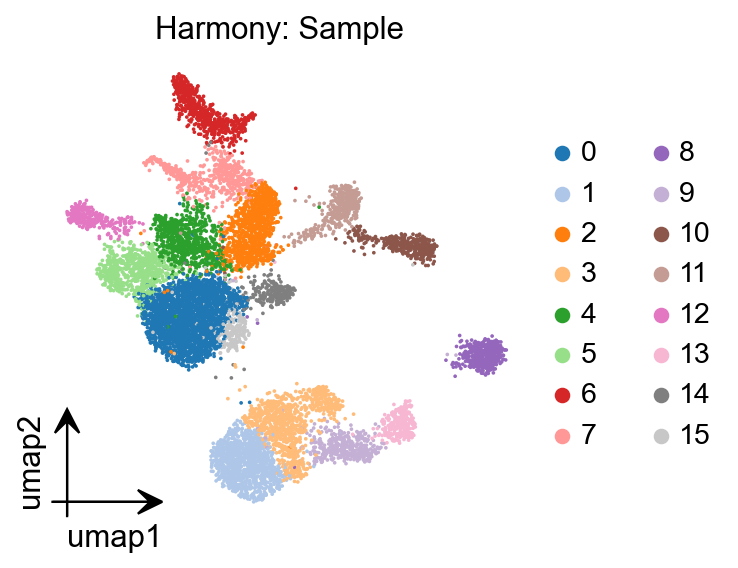
sc.tl.leiden(peak_mat)

running Leiden clustering
finished: found 16 clusters and added
    'leiden', the cluster labels (adata.obs, categorical) (0:00:00)

peak_mat.write('data/pbmc_peak_mat.h5ad')

#peak_mat=sc.read('data/pbmc_peak_mat.h5ad')

Gene Activity

Interestingly, we can also calculate the activity of each gene. For multiple samples, we need to compute them separately and then combine the results.

%%time
# Per-sample gene activity matrix (cached). Barcodes are renamed
# <sample>#<barcode> so the resulting concat lines up with peak_mat.
import pathlib
gene_act_dict = {}
for name in ['scATAC_PBMC_R1', 'scATAC_BMMC_R1', 'scATAC_CD34_BMMC_R1']:
    _cache = f'data/{name}.gene_act.h5ad'
    if pathlib.Path(_cache).exists():
        gene_act_dict[name] = epi.utils.load(_cache)
    else:
        data1 = oom.read(f'result/{name}.h5ad', backed='r+')
        gm = epi.pp.make_gene_matrix(data1, epi.utils.genome.hg19)
        gm.obs_names = [f'{name}#{b}' for b in gm.obs_names]
        gm.obs['sample'] = name
        epi.utils.save(gm, _cache)
        gene_act_dict[name] = gm

└─ loaded AnnData ← data/scATAC_PBMC_R1.gene_act.h5ad  (2496, 20109)
  └─ loaded AnnData ← data/scATAC_BMMC_R1.gene_act.h5ad  (5000, 20109)
└─ loaded AnnData ← data/scATAC_CD34_BMMC_R1.gene_act.h5ad  (3393, 20109)
CPU times: user 87.7 ms, sys: 771 ms, total: 858 ms
Wall time: 888 ms

gene_act_dict

{'scATAC_PBMC_R1': AnnData object with n_obs × n_vars = 2496 × 20109
     obs: 'n_fragment', 'frac_dup', 'frac_mito', 'sample'
     var: 'gene_name',
 'scATAC_BMMC_R1': AnnData object with n_obs × n_vars = 5000 × 20109
     obs: 'n_fragment', 'frac_dup', 'frac_mito', 'sample'
     var: 'gene_name',
 'scATAC_CD34_BMMC_R1': AnnData object with n_obs × n_vars = 3393 × 20109
     obs: 'n_fragment', 'frac_dup', 'frac_mito', 'sample'
     var: 'gene_name'}

gene_act=sc.concat(
    gene_act_dict,
    merge='same'
)
gene_act

AnnData object with n_obs × n_vars = 10889 × 20109
    obs: 'n_fragment', 'frac_dup', 'frac_mito', 'sample'
    var: 'gene_name'

gene_act.obs_names_make_unique()
peak_mat.obs_names_make_unique()

gene_act=gene_act[peak_mat.obs.index]
gene_act.obs['leiden']=peak_mat.obs['leiden']
gene_act.obsm=peak_mat.obsm.copy()
gene_act.obsp=peak_mat.obsp.copy()

%matplotlib inline
epi.pl.umap(
    gene_act,
    #basis='X_umap',
    color='leiden',
    title='Harmony: Sample',
    cmap='RdBu_r',
    vmin=0,
)

gene_act.write('data/pbmc_gene_act.h5ad')

gene_act=sc.read('data/pbmc_gene_act.h5ad')

Preprocess Gene Activity

To do this cell type annotation when we only have scATAC-seq data available, we use prior knowledge of cell type-specific marker genes and we estimate gene expression for these genes from our chromatin accessibility data by uing gene scores. A gene score is essentially a prediction of how highly expressed a gene will be based on the accessibility of regulatory elements in the vicinity of the gene.

sc.pp.filter_genes(gene_act, min_cells=100)

filtered out 2480 genes that are detected in less than 100 cells

# Saving count data
gene_act.layers["counts"] = gene_act.X.copy()
# Normalizing to median total counts
sc.pp.normalize_total(gene_act)
# Logarithmize the data
sc.pp.log1p(gene_act)

normalizing counts per cell
finished (0:00:00)

epi.pl.umap(
    gene_act,
    #basis='X_umap',
    color='CD3D',
    #title='Harmony: Sample',
    cmap='Reds',
    vmin=0,
)

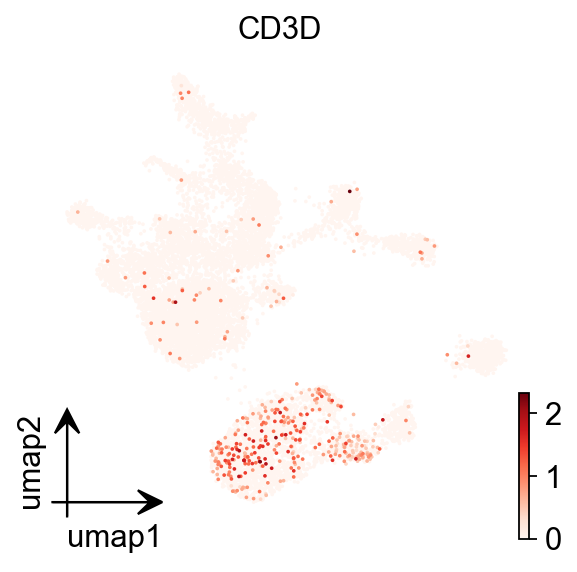
Genes Imputation with MAGIC

In the previous section, you may have noticed that some of the gene score plots appear quite variable. This is because of the sparsity of scATAC-seq data. We can use MAGIC to impute gene scores by smoothing signal across nearby cells. In our hands, this greatly improves the visual interpretation of gene scores.

sc.external.pp.magic(gene_act, name_list="all_genes", knn=5)

computing MAGIC
Running MAGIC with `solver='exact'` on 17629-dimensional data may take a long time. Consider denoising specific genes with `genes=<list-like>` or using `solver='approximate'`.
finished (0:00:57)

epi.pl.umap(
    gene_act,
    #basis='X_umap',
    color='CD3D',
    #title='Harmony: Sample',
    cmap='Reds',
    vmin=0,
)

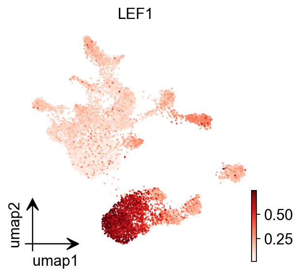
sc.pp.highly_variable_genes(gene_act, n_top_genes=2000, )
gene_act.raw=gene_act.copy()
gene_act=gene_act[:,gene_act.var.highly_variable]
gene_act

extracting highly variable genes
finished (0:00:01)
--> added
    'highly_variable', boolean vector (adata.var)
    'means', float vector (adata.var)
    'dispersions', float vector (adata.var)
    'dispersions_norm', float vector (adata.var)

View of AnnData object with n_obs × n_vars = 10889 × 2000
    obs: 'n_fragment', 'frac_dup', 'frac_mito', 'sample', 'leiden'
    var: 'gene_name', 'n_cells', 'highly_variable', 'means', 'dispersions', 'dispersions_norm'
    uns: 'log1p', 'hvg'
    obsm: 'X_lsi', 'X_lsi_harmony', 'X_umap'
    layers: 'counts'
    obsp: 'connectivities', 'distances'

epi.pl.umap(
    gene_act,
    #basis='X_umap',
    color='LEF1',
    #title='Harmony: Sample',
    cmap='Reds',
    vmax='p99.2',
)

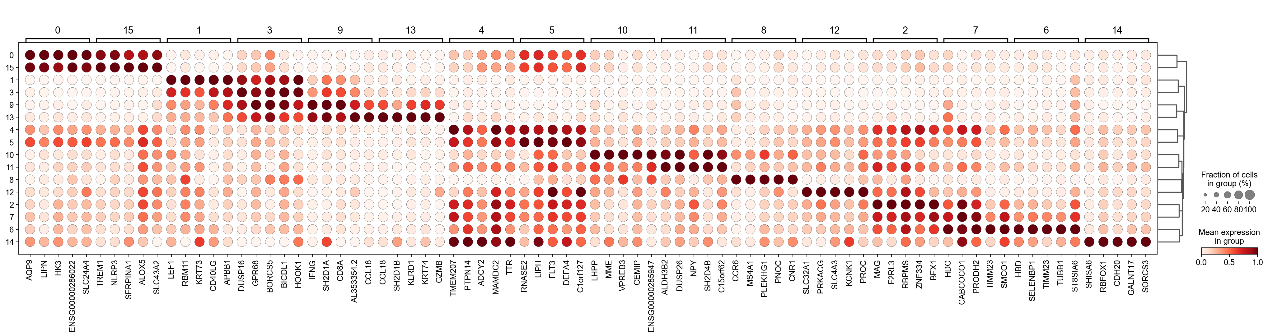
Annotation

# Obtain cluster-specific differentially expressed genes
sc.tl.rank_genes_groups(gene_act, 
                        groupby="leiden", 
                        method="wilcoxon")

ranking genes
finished: added to `.uns['rank_genes_groups']`
    'names', sorted np.recarray to be indexed by group ids
    'scores', sorted np.recarray to be indexed by group ids
    'logfoldchanges', sorted np.recarray to be indexed by group ids
    'pvals', sorted np.recarray to be indexed by group ids
    'pvals_adj', sorted np.recarray to be indexed by group ids (0:00:27)

sc.tl.dendrogram(gene_act,use_rep='X_lsi',groupby='leiden')
sc.pl.rank_genes_groups_dotplot(
    gene_act, groupby="leiden", standard_scale="var", n_genes=5
)

Storing dendrogram info using `.uns['dendrogram_leiden']`

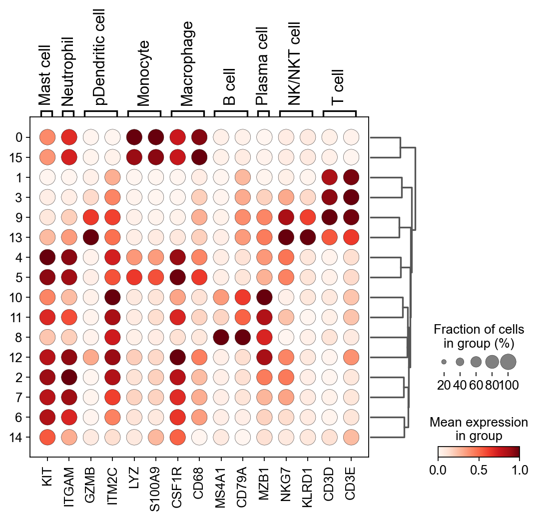
#['CD163', 'CD1C', 'CLEC9A', 'FCGR3B', 'LILRB2', 'S100A12', 'TPSAB1']
small_marker_dict={
    'Fibroblast':['ACTA2'],
    'Endothelium':['PTPRB','PECAM1'],
    'Epithelium':['KRT5','KRT14'],
    'Mast cell':['KIT','CD63'],
    'Neutrophil' :['FCGR3A','ITGAM'],
    'cDendritic cell':['FCER1A','CST3'],
    'pDendritic cell':['IL3RA','GZMB','SERPINF1','ITM2C'],
    'Monocyte' :['CD14','LYZ','S100A8','S100A9','LST1',],
    'Macrophage':['CSF1R','CD68'],
    'B cell':['MS4A1','CD79A'],
    'Plasma cell':['MZB1','IGKC','JCHAIN'],
    'Proliferative signal':['MKI67','TOP2A','STMN1'],
    'NK/NKT cell':['GNLY','NKG7','KLRD1'],
    'T cell':['CD3D','CD3E'],
}
# check if the markers are in the data
smarker_genes_in_data = dict()
for ct, markers in small_marker_dict.items():
    markers_found = list()
    for marker in markers:
        if marker in gene_act.var.index:
            markers_found.append(marker)
    smarker_genes_in_data[ct] = markers_found
#del [] # remove the last marker
del_markers = list()
for ct, markers in smarker_genes_in_data.items():
    if markers==[]:
        del_markers.append(ct)
for ct in del_markers:
    del smarker_genes_in_data[ct]

smarker_genes_in_data

{'Mast cell': ['KIT'],
 'Neutrophil': ['ITGAM'],
 'pDendritic cell': ['GZMB', 'ITM2C'],
 'Monocyte': ['LYZ', 'S100A9'],
 'Macrophage': ['CSF1R', 'CD68'],
 'B cell': ['MS4A1', 'CD79A'],
 'Plasma cell': ['MZB1'],
 'NK/NKT cell': ['NKG7', 'KLRD1'],
 'T cell': ['CD3D', 'CD3E']}

sc.pl.dotplot(
    gene_act,
    groupby="leiden",
    var_names=smarker_genes_in_data,
    dendrogram=True,
    standard_scale="var",  # standard scale: normalize each gene to range from 0 to 1
)

WARNING: Groups are not reordered because the `groupby` categories and the `var_group_labels` are different.
categories: 0, 1, 2, etc.
var_group_labels: Mast cell, Neutrophil, pDendritic cell, etc.

#这是一个空字典用于复制粘贴
cluster2annotation = {
     '0': 'Mono',
     '1': 'T cells',
     '2': 'HSC',
     '3': 'T cells',
     '4': 'CMP_LMPP',
     '5': 'CLP',
     '6': 'Late Ery',
     '7': 'Early Ery',
     '8': 'B cells',
     '9': 'pre-B',
     '10': 'NKT',
     '11': 'pre-B',#CD79A⁺ / MS4A1(CD20)⁻
     '12': 'pDC',
     '13': 'NK',
     '14': 'Endo',
     '15': 'Mono',

}
gene_act.obs['major_celltype'] = gene_act.obs['leiden'].map(cluster2annotation).astype('category')

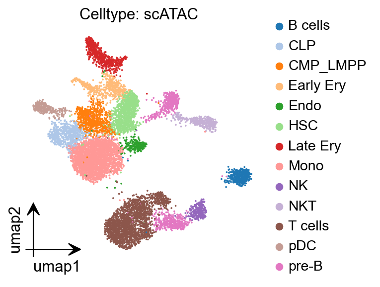
epi.pl.umap(
    gene_act,
    #basis='X_umap',
    color='major_celltype',
    title='Celltype: scATAC',
    cmap='Reds',
    vmax='p99.2',
)

gene_act.write('data/pbmc_gene_act_anno.h5ad')

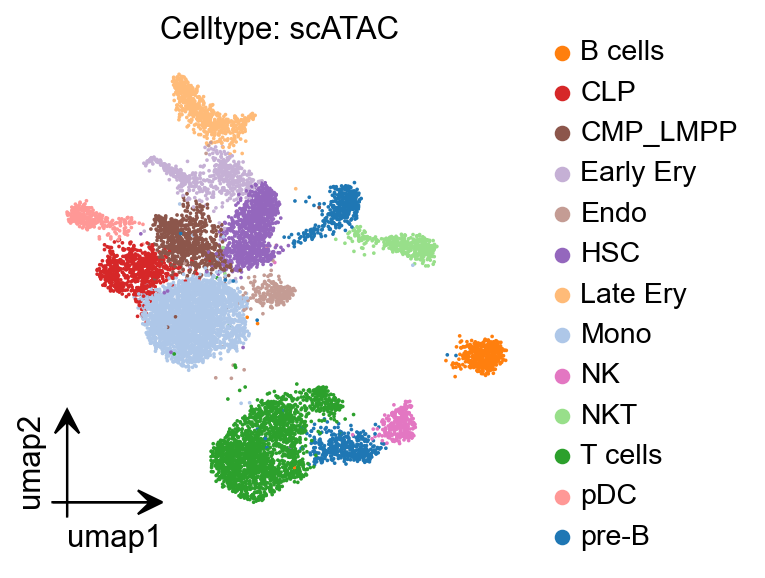
peak_mat.obs['celltype']=gene_act.obs['major_celltype']

epi.pl.umap(
    peak_mat,
    #basis='X_umap',
    color='celltype',
    title='Celltype: scATAC',
    #palette=
    cmap='Reds',
    vmax='p99.2',
)

peak_mat.write('data/pbmc_peak_mat_anno.h5ad')

Peak calling Again

%%time
# Re-use the combined multi-sample AnnData built in Part 2 —
# ``data`` already exists with obs['sample'] and
# uns['files']['fragments'] pointing at the sample#bc-prefixed
# merged fragments file.
data

CPU times: user 4 μs, sys: 0 ns, total: 4 μs
Wall time: 7.39 μs

AnnData object with n_obs × n_vars = 10889 × 0
    obs: 'n_fragment', 'frac_dup', 'frac_mito', 'sample'
    uns: 'files', 'reference_sequences', 'macs3_pseudobulk'

data.obs['celltype']=peak_mat.obs.loc[data.obs_names,'celltype'].tolist()

%%time
# Per-sample MACS3 (cached — delete to force re-run).
import pathlib
_cache = 'data/macs3_per_sample.pkl'
if pathlib.Path(_cache).exists():
    data.uns['macs3_pseudobulk'] = epi.utils.load(_cache)
else:
    epi.single.macs3(data, groupby='sample')
    epi.utils.save(dict(data.uns['macs3_pseudobulk']), _cache)

└─ loaded pickle ← data/macs3_per_sample.pkl
CPU times: user 34.6 ms, sys: 11.9 ms, total: 46.5 ms
Wall time: 49.3 ms

data

AnnData object with n_obs × n_vars = 10889 × 0
    obs: 'n_fragment', 'frac_dup', 'frac_mito', 'sample', 'celltype'
    uns: 'files', 'reference_sequences', 'macs3_pseudobulk'

%%time
merged_peaks = epi.utils.merge_peaks(data.uns['macs3_pseudobulk'], epi.utils.hg19)
merged_peaks.head()

└─ merged 129,750 non-overlapping peaks
CPU times: user 39.7 s, sys: 321 ms, total: 40 s
Wall time: 43.9 s

	chrom	start	end	Peaks	group
0	chr1	565053	565553	chr1:565053-565553	scATAC_PBMC_R1
1	chr1	569133	569633	chr1:569133-569633	scATAC_PBMC_R1
2	chr1	713811	714311	chr1:713811-714311	scATAC_PBMC_R1
3	chr1	752395	752895	chr1:752395-752895	scATAC_BMMC_R1
4	chr1	762612	763112	chr1:762612-763112	scATAC_PBMC_R1

%%time
peak_mat1= epi.pp.make_peak_matrix(data, use_rep=merged_peaks['Peaks'])
peak_mat1

└─ building peak matrix: 10,889 cells × 129,750 peaks
└─ peak matrix nnz=20,701,997
CPU times: user 52.8 s, sys: 2.41 s, total: 55.2 s
Wall time: 55.7 s

AnnData object with n_obs × n_vars = 10889 × 129750
    obs: 'n_fragment', 'frac_dup', 'frac_mito', 'sample', 'celltype'
    uns: 'files', 'reference_sequences'

Since we are using anndata-rs to read data stored on the hard disk, we need to perform a close operation to ensure data integrity and security.

# data.close() not needed for anndataoom — backed writes are flushed.

peak_mat1.obsm=peak_mat.obsm.copy()
peak_mat1.obsp=peak_mat.obsp.copy()

epi.pl.umap(
    peak_mat1,
    #basis='X_umap',
    color='celltype',
    title='Celltype: scATAC',
    #palette=
    cmap='Reds',
    vmax='p99.2',
)

peak_mat1.write('data/pbmc_peak_calling.h5ad')